


The GENESYS (Generation Evaluation System) model was developed to assess the adequacy of the Pacific Northwest regional power supply, given uncertain future conditions. It is also the primary analytical tool the Council uses to quantify the impacts of modifying hydroelectric system operations (e.g., to accommodate the changing needs of all river users). GENESYS is a constrained economic dispatch model that uses Monte Carlo sampling to assess the effects of uncertainty in demand, stream flows, wind and solar generation and generator forced outages. The model simulates the dispatch of hydroelectric projects and other generating resources in a multi-stage process to emulate real-life electric utility decision making and operations.
Background
Prior to 1999, future resource needs were estimated by calculating the power supply’s load-resource balance.[1] This type of calculation is usually made for both energy and capacity needs. Energy needs refer to having sufficient generating capability and fuel to match annual average demand, in units of megawatt-hours (or average megawatts). Traditionally[2], capacity needs refer to having sufficient generating capacity to match the highest single-hour demand during the year, in units of megawatts. Using this approach, the implied objective is to have sufficient energy and capacity generating capability to serve the expected annual average demand and the year’s highest single-hour demand, with sufficient reserves to cover resource outages, temperature fluctuations and variations in renewable resource generation.
Generally, the load-resource balance only includes existing resources and critical year[3] hydroelectric generating capability but does not include market supply, thus making it a conservative estimate of resource needs. Planners have generally agreed that a deficit load-resource balance does not automatically imply an inadequate power system because in-region and out-of-region market supplies could often make up the difference and the likelihood of a critical water year is relatively low (about two percent). By 1999, however, due to little resource development during the decade, the load-resource balance deficit had become alarmingly large. And, because the load-resource balance does not provide any insight into the probability of potential shortfalls, there was a general concern as to whether the power supply was adequate.
To address this concern and to assess resource adequacy more quantitatively, the Council turned to probabilistic methods. In conjunction with regional stakeholders, in 1999 the Council developed the GENESYS model, which utilizes stochastic variables to perform a hydroelectric and thermal generation dispatch. GENESYS was not designed to address long-term load uncertainty and thus, does not employ system expansion logic. That function is included in the Council’s resource expansion model, the Regional Portfolio Model (RPM), which uses adequacy thresholds (adequacy reserve margins) derived from the GENESYS analysis to ensure that resource strategies will provide adequate supplies.
GENESYS simulates the operation of the region’s power system on a multi-stage basis (described in more detail below) while meeting all system requirements for energy, capacity, and ancillary services. It also adheres to resource operating constraints, including hydroelectric operations mandated by the Council’s Fish and Wildlife Program and by the Endangered Species Act. It dispatches resources based on need or when economic to do so, based on operating costs relative to market prices. Economic dispatch of hydroelectric projects is based on a projected value of water behind the dams. GENESYS records all hours when load cannot be fully served and produces outputs which analysts use to identify underlying causes (i.e., river flow, demand, wind and solar generation and generator forced outages).
The Pacific Northwest power supply has traditionally been considered to be capacity surplus because of the high nameplate capacity of its hydroelectric system relative to its fuel supply (river flow volume). For example, its aggregate nameplate capacity is about 35,000 megawatts whereas, in an average water year, it only produces about 16,000 average megawatts of energy. Since the 1980s, however, growing restrictions on hydroelectric operations combined with rapid increases in variable energy resources (wind and solar) and more complex market dynamics have made the region more susceptible to capacity shortfalls. Because of this, the GENESYS model was redeveloped to enhance its analytical capabilities for assessing energy and capacity needs and to structure the code base to simplify future development and maintenance. The table below summarizes key enhancements, relative to the original GENESYS model.
Key GENESYS Enhancements
| Redeveloped GENESYS | Original GENESYS |
| 17 regional zones and 16 zones outside the region with interconnecting transmission | 2 regional nodes (east and west) with interconnecting transmission |
| Dynamic WECC-wide market price and supply, economic market sales | Fixed user-defined market price and supply, no market sales |
| Hourly dispatch of individual hydroelectric projects | Hourly dispatch of aggregate hydroelectric system |
| Multi-stage resource unit commitment | Simplified day-ahead unit commitment for coal plants only |
| Dynamic allocation of contingency and operating reserves | Checks for ability to provide contingency reserves post-dispatch, fixed allocation of hydroelectric balancing reserves, no allocation of thermal resource reserves |
| Dynamic assessment of the value of water in reservoirs | Fixed value of water in reservoirs |
| Optimization to minimize cost | No explicit optimization, dispatch based on resource cost |
In its optimization, the redeveloped GENESYS prioritizes key monthly and hourly hydroelectric operating constraints by assigning each a penalty. However, due to power plan timing constraints and in lieu of having to input and fine-tune the penalties for the thousands of monthly hydroelectric operating constraints fed into the original GENESYS,[4] the resulting end-of-month[5] project elevations from an original GENESYS analysis are used as target elevations in the redeveloped model for supporting the power plan analysis. This method allows the redeveloped model to adhere to Canadian hydro operations (as defined under the Columbia River Treaty).
There is a brief discussion below of the differences in model logic between the redeveloped and classic GENESYS, but the redevelopment process and public vetting is catalogued in more detail at the following sites:
System Analysis Advisory Committee Meetings
The redeveloped model uses a multi-stage decision making process (like in the original GENESYS) but adds forecast error and more advanced commitment logic in addition to a deployment (true up) stage after the weekly, day-ahead, and hour-ahead stages are completed. The weekly stage assesses average energy dispatch for the week. The day-ahead commitment stage uses forecasted demand and prices to commit generating resources for the next day and optimizes the forecasted hourly operation over a week. It is performed every 24 hours on a “rolling” basis. The hour-ahead commitment stage optimizes the hourly forecasted operation over a day and is performed every hour. The deployment stage determines the “actual” operation in an hour using “observed” demand and variable energy resource generation.
The figure below is a graphic showing the time stages. The stages in blue are optimizations. For a mathematical description of equations, see the documentation on the Council website.
Multi-Stage Resource Commitment

Weekly Stage
The weekly-stage logic for the redeveloped GENESYS is similar to the original GENESYS monthly-stage logic. In the original model, a water year is divided into 14 periods which are, for the most part, monthly, with April and August split into two separate periods. The 14-period hydro regulator algorithm used to determine available hydroelectric generation in the original GENESYS is the same logic found in the Bonneville Power Administration’s HYDSIM model. Reservoir operating constraints include minimum and maximum flow, minimum and maximum storage, and minimum and maximum spill at each hydro project for each of the 14 periods. For each period, the amount of hydro energy available to each regional zone is calculated and separated into “blocks” of energy with different monetary values. For example, water above the flood control elevation (maximum storage) is very inexpensive since it must be evacuated by the end of the month regardless of market price. Water between the flood control elevation and the refill elevation (target elevation that ensures a high likelihood of refill by specified date) is moderately valued because it can be held in storage or drafted depending on market price. Water between the refill elevation and the contractual drafting rights elevation (lowest elevation for optimal operation) is higher valued and should be held in storage if cheaper resources are available. Finally, water below the drafting rights elevation is very expensive because using it will jeopardize the adequacy of the power supply in later periods.[6] It should be noted that water below the drafting rights elevation (referred to as “borrowed” hydro) can be used for short durations to increase hydro flexibility, as long as it is promptly replaced. Modelers refer to the flood control elevation as the Upper Rule Curve[7] (URC), to the refill elevation as the Variable Energy Content Curve[8] (VECC), to the drafting rights elevation as the Proportional Draft Point (PDP).
Hydro block 1 is the amount of energy that must be generated to get to URC plus the energy generated by the hydro independents.
Hydro block 2 is the amount of energy between URC and VECC.
Hydro block 3 is the amount of energy between VECC and draft point 6.
Hydro block 4 is the amount of energy between draft point 6 and CRC, Critical Rule Curve[9].
Hydro block 5 is the amount of energy between hydro block 4 and draft point 8, limited by the user input for “borrowed hydro” of a 1000 MW-periods. Draft point 8 is the total energy when drafting from starting content to as close to empty as constraints allow.
The hydro blocks are divided between the zones in the Pacific Northwest region according to the total amount of hydro energy output from the hydro projects specified for each zone.
In the original GENESYS, the monetary values (shadow prices) of hydro blocks are provided by the user. Shadow prices are used to determine hydro block dispatch order relative to other generating resources. However, in the redeveloped GENESYS, the hydro is not broken into specific blocks and the shadow prices are dynamically assessed using an algorithm that determines the current period’s value of water given the objective to refill the reservoir system to a desired elevation by a specified future date[10] given the other constraints on the river.
This shadow price (also referred to as the “future value of water”) in the redeveloped GENESYS is calculated given a target date to get the system to the desired storage considering a distribution of inflow uncertainty between the current and target dates. It can be calculated forward in time from any period and system content to the target date and desired system storage. This expected future value of water is calculated incorporating inflow uncertainty, meeting the load during the period, and ending up at the storage target. For example, say we calculate a future value of water at the beginning of January given that we need to fill by the end of July. The algorithm starts by calculating a value for any system content at the beginning of July to meet the load and end full at the end of July. Once that is calculated, the same process is completed for June, minimizing costs given the uncertainty of inflows to meet the previous period load. This process continues until we get to the time step of interest (in this case January). The future value of hydro is determined for each period in units of $/MW-month.
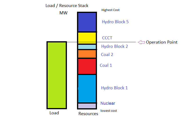
The original GENESYS does a period economic average energy dispatch by node[11] using an algorithm that mimics what is shown in the figure below. After dispatching resources within each node for the node’s load, it finds “opportunities” in each of the nodes for displacement of resources or the meeting of load that was not served by the node’s own resources. It then goes through the resources not yet dispatched by economic order and determines, given economics and transmission constraints, whether that resource supplies any of the “opportunities”. This results in an economic dispatch of the region’s resources, given transmission constraints between the nodes.
Load/Resource Stack in GENESYS Period Dispatch
The original GENESYS, after going through the period dispatch, week dispatch, day dispatch, and hour dispatch for the entire month, calculates the total amount of hydro energy dispatched in the month and the hydro regulator is run again to determine the ending contents of the reservoirs for that month, which become the starting contents for the next month. The redeveloped GENESYS does not need to go through this type of process to calculate end-of-month reservoir elevations, since the elevations in the last hour’s deployment stage are the starting elevations for the next stage.
Commitment Stages (Week and Day)
Redeveloped GENESYS optimizes the use of available hydro storage and thermal resource operation given forecasted river flows and demand over the coming week, by hour, to minimize costs to meet system requirements. In addition, when necessary to maintain adequacy or when prices are advantageous, it can commit coal and gas-fired resources for next day operation keeping in mind their planned operation for the coming week. It revisits this commitment decision every day on a rolling basis. Resources are modeled individually, including all regional hydroelectric facilities. The resulting operation takes into account the interaction among all power supply components; hydro and thermal resources, variable energy resources (like solar and wind), energy limited resources (like demand response and storage) and must-take resources (like long-term contracts). The system requirements include:
- Base Load[12]
- Regulation up
- Imbalance up
- Regulation down
- Imbalance down
- Spinning reserve
- Non-spinning reserve
The model is formulated to explicitly model the holding of reserves by specific plants and the determination of whether those reserves are used is made in the deployment stage. The summation of all held capacity reserves for a particular requirement must meet the total system requirement. The optimization is over the total WECC, but the resources are modeled in more detail within the region[13].
Objective Function
The objective function minimizes cost. This includes fuel costs, variable O&M costs, wear and tear costs, and startup costs of resources. Total cost also includes penalties for violating operating constraints and for forced spill at hydro projects and also accounts for the future value of resources[14]. Figure 4 is a graphical representation of the tradeoff between immediate thermal costs and storing water versus drafting hydro and running thermal resources in the future.
Thermal Resources
Thermal resource operation is limited by ramping capability, minimum operating level, and maximum capacity. If a coal plant or combined cycle combustion turbine is forecast to be needed in the next day, or if a natural gas peaking plant is forecast to be needed in the next hour, it is committed for potential operation. If a resource is committed, its operation is constrained by its minimum generation requirement, its fuel schedule and its minimum and maximum fuel usage deviation from schedule[15]. A plant may also be constrained by minimum up and down time requirements.
Hydro Resources
Hydro resource operations are constrained by their maximum capacity, ramp up and down rates and by their minimum generation requirements (i.e., minimum turbine flow). Total outflow (scheduled turbine flow plus discretionary and forced spill) is constrained by minimum and maximum outflow requirements for each project. Achieving discretionary spill target flows is dependent on having sufficient inflow and reservoir storage to first meet the minimum turbine flow requirement. The discretionary spill target (by period for fish survival) can be a fixed flow rate or can be a percentage of total outflow. Reservoir volumes are constrained by minimum and maximum elevation limits, both physical (absolute top and bottom) and operational (to maintain specific lake levels or for other considerations).[16] River inflow into each reservoir is the sum of outflows from all upstream reservoirs plus side flows. The outflow at each reservoir is its inflow plus water that is drafted or minus water that is held to fill the reservoir.
The computation of generation from a hydro project is a non-linear function of the forebay elevation, tailwater elevation and turbine flow. Conversion factors (H/K) of hydro projects vary by net head (forebay elevation minus tailwater elevation).
Variable Energy Resources
Variable energy resources, such as wind and solar, can be dispatched down to alleviate oversupply. Maximum hourly generation from these resources is determined exogenously, either from historical data or from forecasts (of wind speed and direction or of solar availability). Generation from these resources is dispatched down if not needed to serve demand or if it is uneconomical in the open market. Hourly generation capacity factors[17] for an entire year are provided for multiple years (with each year having different hourly wind and solar patterns).
Energy Limited Resources
Energy limited resources are limited by a total number of megawatt hours stored. The resource can choose to store or generate in any given hour. The maximum amount of capacity held on a particular energy limited resource must be less than or equal to its maximum capability and what is available per the energy stored.
GENESYS optimizes the planned use of hydro and thermal resources, including reserves, over the next day, by hour, to minimize cost. It does this by three-hour blocks on a rolling basis through the entire day. The commitment of short-term plants such as gas-fired turbines is re-examined at each hour. Constraints are essentially the same as for the day-ahead stage but cover a different time period. Simulated forecasts for demand and variable energy resource generation are revised to reflect the improvement of forecasts over time.
This stage models operations that are taken to resolve differences between forecasted parameters (demand, wind and solar generation, etc.) used in the hour-ahead stage and actual parameters “observed” in this hour. Actual utilization of all resources will be determined, including the use of reserves. In this stage, a stochastic determination of thermal plant availability is made and an accounting of fuel use is made.
Note About Transmission in the Redeveloped Model
For the purposes of the plan studies, net imports into the region were limited [18] but power could still utilize transport capability of the transmission lines for power to flow through the region. For example, if BC Hydro wanted to import 100 MW of power in one hour from the CAISO, that power would have to be transmitted through the region. While the imports to the region would be 100 MW from CAISO, the exports would also be 100 MW, and thus the net imports would be 0 MW in that hour.
Additionally, if a remote regional resource[19], say Jim Bridger Unit 3, was not utilizing all of its firm rights to transmit power the assumption was that other resources could use those rights if available[20]. This more detailed way of modeling the transmission system was discussed extensively in the System Analysis Advisory Committee and Resource Adequacy Advisory Committee.
[1] Load-resource balances are estimated and published in the PNUCC NRF and the BPA White Book.
[2] Capabilities are now often evaluated against net peak need which is sometimes evaluated by the largest demand net variable generation residual in any particular hour.
[3] Generally, the term “critical year” refers to the annual streamflow record that produces the lowest hydroelectric generation.
[4] Ultimately, the redeveloped GENESYS will incorporate all binding constraints, thus making this step in the process obsolete. In the interim, this step was taken to both simplify and expedite completion of the model and to aid in the vetting process.
[5] The original GENESYS model split April and August into two separate periods to account for river flow ramp up period in April and the ramp down period in August.
[6] Because of constraints other than the rule curves, GENESYS never gets to empty.
[7] Upper Rule Curve is also known as the flood control rule curve. Calculated by the Army Corp of Engineers, it “defines the drawdown required to assure adequate space is available in a reservoir to regulate predicted runoff for the year without causing flooding downstream.”, per “Modeling the System” pamphlet.
[8] Variable Energy Content Curve guides non-firm generation energy generation, and is usually the lowest of the four rule curves in winter and early spring and is based on the predicted runoff during the year. Functionally this is a reservoir energy content curve. Drafting a reservoir no further than this point ensures a high probability of refilling by the end of spring runoff season. VECC is made up of Made up of the Assured Refill (ARC), Variable Refill (VRC), and Limiting Rule (LRC) Curves from BPA
[9] Critical Rule Curve “defines the reservoir elevations that meet firm energy hydro requirements under the most adverse stream flows on record”, per “Modeling the System” pamphlet.
[10] See Discussion of Future Value in Day-Ahead Commitment Stage.
[11] Note that in the revised version of GENESYS, “nodes” are now referred to as “zones.”
[12] The base load plus regulation down and imbalance down requirements equals the scheduled load.
[13] Recall that the region consists of all the loads and resources within each zone of the region and transmission constraints between the zones.
[14] This is treated as the “fuel” cost of hydro
[15] Drafting and packing of the gas pipeline for gas.
[16] Storage targets can be modeled as a range of possible values that narrows as it approaches the target date.
[17] Hourly generation for wind and solar resources is equal to the hourly capacity factor time the installed nameplate capacity.
[18]See the Market Supply Assumptions table.
[19] A generator that is sited remotely but is considered a regional resource.
[20] The mechanism that this process in the model is emulating is primary or secondary transmission sales. This usually happens via a coordinated scheduling process in which a party that owns firm transmission rights sells, on a short-term basis, the right to transmit power across those lines.