


The energy use forecast models are based in part on historical temperatures at four sites throughout the region. The data used are from the National Oceanic and Atmospheric Administration’s (NOAA) Climatic Data Online system, in particular the Local Climatological Data published on that system contains hourly observed temperatures.
- Boise Airport
- Portland International Airport
- Seattle-Tacoma International Airport
- Spokane International Airport
The models use data that range from 1948 to 2018.
Regional Temperature Calculation
Regional temperatures are calculated based on a legacy regression. This is done for consistency with previous plans and regional analyses. To calculate the regional average temperature, we use the following formula:
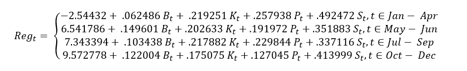
Where t is a historic hour and at hour t , Bt is the temperature in Boise, Kt is the temperature in Spokane, Pt is the temperature in Portland, and St is the temperature in Seattle.
The result of this calculation is equivalent to a weighted average temperature on a partition of the set of historic hours.
Principal Component Analysis
While we did not update the calculation for the plan to preserve backward compatibility, we did some verification (R script file) to make sure a weighted average was a reasonable representation. We know that these data are highly correlated and thus there is substantial collinearity between the temperatures when included together in a regression model. For example, the following correlation matrix is calculated with the data from 2008 to 2018:
| Boise | Portland | Seattle | Spokane | |
| Boise | 1.000 | 0.888 | 0.879 | 0.938 |
| Portland | 0.888 | 1.000 | 0.934 | 0.889 |
| Seattle | 0.879 | 0.934 | 1.000 | 0.914 |
| Spokane | 0.938 | 0.889 | 0.914 | 1.000 |
Principal component analysis allows for calculating transformations of these data that are independent. By looking at the principal components we can evaluate what combination of these temperatures is likely to capture the structural relationship between these variables and able to best represent the span of these data. For example, if we run a principal component analysis on the January through April data (to be consistent with the legacy temperature partition described above), we get the following principal components:
| PC1 | PC2 | PC3 | PC4 | |
| Boise | 0.623977 | 0.502471 | 0.573248 | -0.17194 |
| Spokane | 0.56347 | 0.240399 | -0.74421 | 0.266189 |
| Portland | 0.421564 | -0.67421 | 0.291574 | 0.531706 |
| Seattle | 0.339762 | -0.48495 | -0.18033 | -0.78541 |
Where PC1 is the component that captures the most variation and each component, in this case it explains just over 84 percent of the variance. PC2 through PC4 explain the variance in descending order. For this example, PC2 explains just over 8 percent of the variance and PC3 explains slightly less than 6 percent.
Another way to interpret this is to say that the most important information looking at the four temperature measurements is an average of all four temperatures which by far explains the most structural variance in these data. After that, the next most important information the difference between the observations on the eastside of the region and the westside of the region. And closely following that is looking at the difference between the temperatures in the northern part of the region and the southern part of the region.
Principal components create a transformed basis for these data. That is, each component can be thought of as a vector. Thus, the first component can be transformed into a weighted average. This is one data driven approach to forming a weighted average that accommodates the collinearity of these data. For this example (January through April of 2008 through 2018), the weights would be:
| Boise | Spokane | Portland | Seattle |
| 32.0% | 28.9% | 21.6% | 17.4% |
The weights depend on years selected and the months analyzed, but given the high correlation between the temperature observations, it’s likely that different similarly reasonable weighting schemes would not substantially change the results when used in a regression setting. In fact, for the example examined, a regression with regional historical load as the response variable using just the first principal component has about a 1 percent increase in the SSE (sum of squared error) compared to a simple additive model for these temperature data.