


This section describes an R-script that transforms the AURORA output for the Western Electricity Coordinating Council (WECC) generation capability and dispatch cost into available import power market supply and associated power prices for the Northwest for input into the redeveloped GENESYS model.
The figure below shows a few rows of an example AURORA output that has about 54 million rows of hourly generation capabilities and dispatch costs for a calendar year and for the 46 zones in WECC (see AURORA write-up for more details).

A portion of an example AURORA output of hourly generation capabilities (column G in MW) and dispatch costs (column H in $/MW-hour)
In the above table, column A identifies the AURORA WECC zone, which for the rows presented is Alberta. Then columns B to E specify respectively the year, month, day and hour being modeled in AURORA. Next, column F lists the names of specific power plants. Then column G specifies the generation capability of the corresponding power plant in column F, in units of MW. Finally, column H lists the dispatch cost for the corresponding plant in column F, in units of $/(MW*hour) . For example, the first 58 power plants, listed in cells F2 to F59, all have the same negative dispatch cost at -24.381 $/(MW*hour) .
The WECC generation capability and associated dispatch cost data are then transformed and formatted into inputs file for the redeveloped GENESYS (which henceforth simplifies to just GENESYS) to model power market import into the Northwest.
However, GENESYS has 19 WECC buses (in contrast to the 46 AURORA zones see redeveloped GENESYS write-up for more details). The figure below lists the 46 AURORA zones and their corresponding 19 GENESYS buses.

The 46 AURORA zones and corresponding 19 GENESYS buses
Since the generation capability and cost data in the AURORA output are used to model market import into the Northwest, which is designated by the GENESYS bus PNW in the above table, then data from those AURORA zones that correspond to the PNW bus are excluded from the calculations.
There are also a few power plants in some GENESYS (non PNW) buses where a portion of their capabilities already serves the regional Northwest load, thus only the remaining portion is available for the import market. Hence, a multiplicative factor for each power plant in column F in the previous figure is used to adjust the corresponding capability in column G.
Moreover, power plants with dispatch costs in column H greater than 500 $/(MW*hour) are considered emergency resources in the corresponding AURORA zone, and thus those plants are also excluded from market import calculations for the Northwest.
Furthermore, in contrast to the granular dispatch cost in the first table, each GENESYS bus has power prices grouped into its own specific number of price bins. For example, the GENESYS Alberta bus has 13 price bins, Alberta_0, Alberta_20, Alberta_30, Alberta_40, Alberta_50, Alberta_60, Alberta_70, Alberta_80, Alberta_90, Alberta_100, Alberta_110, Alberta_120, Alberta_460. More specifically, the Alberta_0 bin represents prices <0 $/(MW*hour) ; the Alberta_20 bin represents prices for which 0 $/(MW*hour) ≤ prices <20 $/(MW*hour) , and so on. There are a total of 384 price bins for the 18 non-PNW GENESYS buses in the above figure.
Therefore, to enable transforming the AURORA output data into appropriate GENESYS inputs, the multiplicative factor for each plant, the GENESYS buses and their corresponding price bins are merged into the AURORA data by an R-script, which results in the table below.

A portion of an example AURORA output are merged with corresponding GENESYS buses (column B) and price bins (column J)
Because of horizontal space limit, the multiplicative factors are not shown above but they have been used to modify the generation capabilities in column H. For the plants listed, all the factors are 1.
Thus, for each month, day and hour and each GENESYS price bin (column J) in each GENESYS bus (column B), the R-script calculates the sum of all the corresponding modified capabilities in column H. For example, for the GENESYS Alberta bus and the Alberta_0 price bin, and for Month = 1, Day = 1 and Hour = 1, let the generation capability of the 58 plants in the Alberta_0 bin, in cells H2 to H59, be represented by C1 to C58 respectively. Then the sum of all the modified capabilities for the Alberta_0 bin is
The sums of modified capabilities for other GENESYS buses and price bins and other months, days and hours are similarly calculated. The result, in GENESYS input format, is presented below.
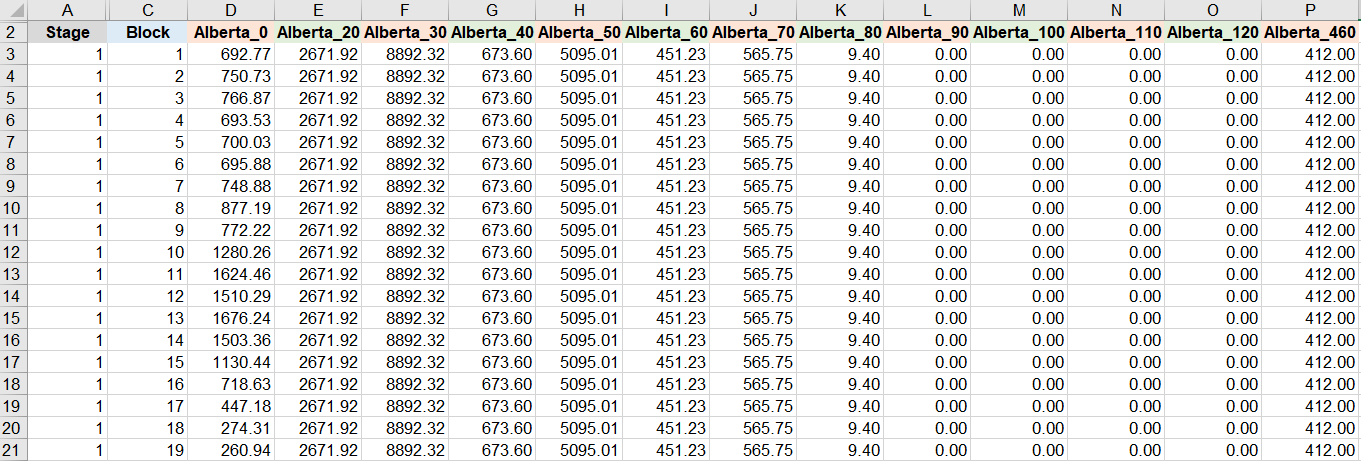
A portion of the sum of capabilities for each GENESYS price bin and each GENESYS bus. Data for the 13 Alberta price bins in the Alberta bus are listed in columns D to P
In the above table, the Stage column (A) lists the weeks, with a range from 1 to 52, of the calendar year and the Block column (B) indicates the hour index of each week, with a range from 1 to 168. After the Block column, there are 384 columns of capability sums for all the price bins of the 18 non-PNW GENESYS buses listed above.
For example, for the first hour of the first week (Block = 1, Stage = 1) of the calendar year, the capability sum for the Alberta_0 price bin is 692.77 MW in cell D3, as previously calculated. Furthermore, for the data presented, the highest generation capability in the Alberta bus is 8,892 MW for the Alberta_30 bin (column F) where the price range is 20 $/(MW*hour) ≤ prices <30 $/(MW*hour) . In contrast, there is no generation capability for the four bins, Alberta_90, Alberta_100, Alberta_110 and Alberta_120, in columns L to O respectively.
Finally, a capability-weighted average dispatch cost for all power plants in each GENESYS price bin for each GENESYS bus and for each month, day and hour is also calculated by the R-script. For example, for Month = 1, Day = 1 and Hour = 1, and for the Alberta_0 bin, let C1 to C58 , corresponding to cells H2 to H59 respectively, represent the generation capability of the 58 plants listed in cells F2 to F59. Also, let D1 to D58 , corresponding to cells I2 to I59 respectively, represent the dispatch costs of the 58 plants. Then, the capability-weighted average dispatch cost for the Alberta_0 bin is
For those price bins where the denominator, the capability sum, is 0, then the average dispatch cost is also 0. The capability-weighted average dispatch costs for other GENESYS buses and price bins and other months, days and hours are similarly calculated. The result, in GENESYS input format, is presented below.
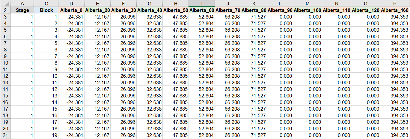
A portion of the capability-weighted average dispatch cost for each GENESYS price bin and each GENESYS bus. Data for the 13 Alberta price bins in the Alberta bus are listed in columns D to P
In the table above, the columns have the same representations as those in the previous table, where the Stage column (A) lists the weeks of the calendar year and the Block column (B) indicates the hour index of each week. Furthermore, after the Block column, there are 384 columns of capability-weighted average dispatch cost for all the price bins of the 18 non-PNW GENESYS buses.
For example, for the first hour of the first week (Block = 1, Stage = 1) of the calendar year, the capability-weighted average dispatch cost for the Alberta_0 price bin is -24.381 $/(MW*hour) in cell D3, as calculated previously. Furthermore, for the data presented, the capability-weighted average dispatch cost is 12.167 $/(MW*hour) for the Alberta_20 bin (column E).