


As discussed above, the Council has developed a method to assess the effective generating capability for sets of resource portfolios. This differs from what was done in the past, when effective capacity was assessed for individual resources only. While this information is invaluable to system planners in terms of quantifying each portfolio’s effectiveness toward meeting adequacy needs, by itself it does not provide any insight as to the most cost-effective mix of new resources to meet those needs. To determine cost-effective sets of resource portfolios, the Council relies on its Regional Portfolio Model (RPM). The RPM is a system expansion model that acquires new resources over a 20-year study horizon, considering a wide range of future demand growth paths along with other uncertain future conditions. The RPM will acquire resources if they are expected to be profitable, if they are required by policies and/or if they are needed to maintain adequacy. In order to accurately size new resources, the effective capability of a resource or of a resource mix must be known to ensure that the model does not under or overbuild. Effective resource capability is assessed by determining how much additional demand can adequately be served by an increment of new resource. The metric the Council uses to quantify effective capability is referred to as the Associated System Capacity Contribution (ASCC) and is measured as the percentage of nameplate capacity that can be counted on toward meeting the adequacy reserve margin (ARM) requirement.
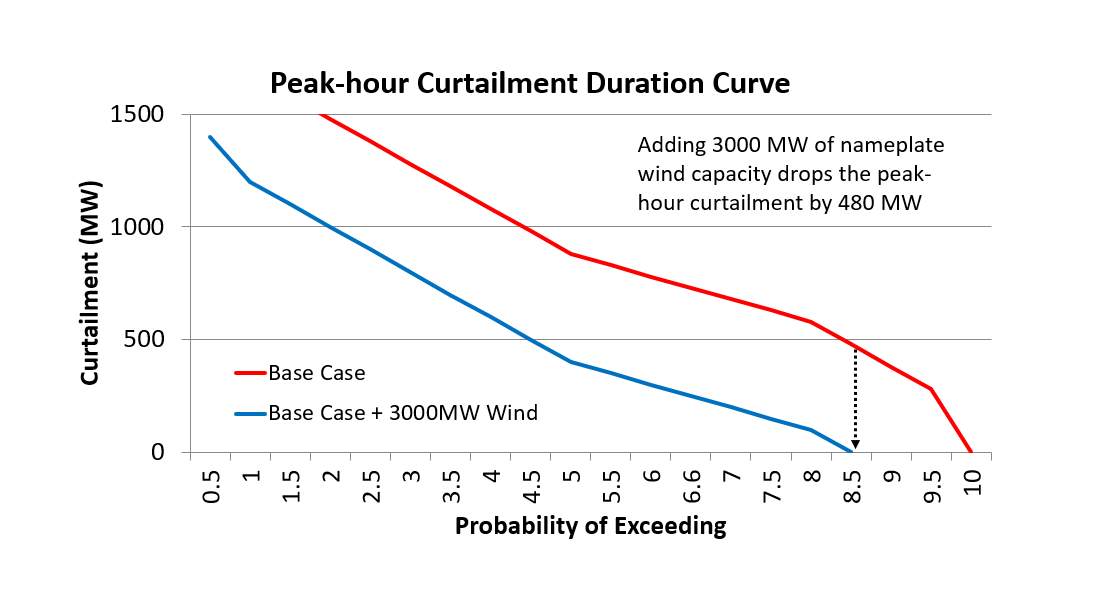
A more commonly used metric is the Effective Load Carrying Capability (ELCC), which may provide a more accurate estimate of effective capacity but generally involves multiple iterative studies. The ASCC differs from the ELCC in that it only requires one additional study. This is critical for the Council’s work because of the high number of ASCC assessments needed for the expansion model (see below). Additionally, to have used ELCC would have required a more granular adequacy metric or target such as expected unserved energy by quarter. The ASCC is calculated by measuring the decrease in the peak-hour curtailment duration curve when a resource is added to a base case.[1] The peak-hour curtailment duration curve is the set of every simulation’s highest hourly curtailment, sorted from highest to lowest. For illustration, an example of a peak-hour curtailment duration curve is shown in the figure below. Since each simulation has the same likelihood of occurrence, the x-axis represents the curtailment exceedance probability and the point at which the curve crosses zero is the loss of load probability (LOLP). In this example, adding 3,000 megawatts of wind nameplate capacity dropped the LOLP from 10 percent to 8.5 percent. The ASCC for this wind resource is equal to the decrease in peak-hour curtailment (480 megawatts) divided by the installed nameplate capacity (3,000 megawatts) or 16 percent. In other words, this 3,000 megawatt nameplate capacity wind resource, when added to the base case supply, provides 480 megawatts of effective system capability.
Resource portfolio ASCCs are calculated in the same way. More precisely, quarterly ASCC values used in the RPM are calculated using the deficit record from two studies as follows:
The ASCC is calculated for a particular set of resources is defined using the deficit record from two studies as follows:
- Define peak needs before adding resources
Base run maximum deficits by game g and quarter q
Max(DeficitsBase)g,q
- Define peak needs after adding resources
Run with capacity added maximum deficits by game g and quarter q
Max(DeficitsResourceAdd)g,q
- Peak needs reduction by adding resources
∆g,q=Max(DeficitsBase)g,q-Max(DeficitsResourceAdd)g,q
- Expected peak needs contribution from adding resources
Take the expected value of those differences over all the game g and quarter q, ∆g,q and divide by the total size of resource strategy, R[1], that is selected to test in RPM
E(∆g,q) /R
As is well known, effective resource capacity varies with the amount of new resource added and varies based on the overall resource mix. In the past, the Council has calculated the ASCC for individual resource types as a function of added resource nameplate capacity. While this accounts for the decline in ASCC when more of a particular resource is added, it does not address the decline in ASCC when other types of resources are added. To resolve this issue, the Council developed a method to assess the ASCC for sets of resource portfolios. Each portfolio has a different mix of resources with differing amounts of added capacity. By creating an ASCC array that covers a wide range of resource types and added capacities, the ASCC for a possible future resource portfolio can be estimated by interpolating between the two closest points in the ASCC array.
The ASCC array provides a more accurate estimate of the amount the existing portfolio’s effective capability increases than using individual resource ASCC values. For example, consider portfolios that in addition to 300 average megawatts of additional energy efficiency[3] include, a 5,000-megawatt solar resource and a 3,000-megawatt wind resource. The fall[4] ASCC for the solar resource is estimated to be about 25 percent and the fall ASCC for the wind resource is estimated to be about 16 percent. Simply summing the effective capabilities based on those ASCC values would result in 1,730 megawatts (5000 x 0.25 + 3000 x 0.16) predicted additional capability in fall. However, the portfolio ASCC for the combination of 5,000-megawatt solar resource and a 3,000-megawatt wind resource is 14 percent, which leads to an additional effective capability of 1,120 megawatts (8000 x 0.14). Thus, for this example, summing the individual ASCC values overestimates the effective capacity of the solar/wind portfolio by 610 megawatts and would lead to underbuilding (and potentially an inadequate supply).
In theory, an ASCC array can be thought of as a multidimensional surface with each axis representing a different resource. The composite ASCC for a set of new resources is that point on the surface defined by the amounts of new resources added along each axis. If we have 7 resource types in our supply curve, that means that our ASCC surface will have 8 dimensions (the 8th dimension is the composite ASCC value). It was not feasible to derive an equation for the composite ASCC as a function of the amounts of new resources added within the timeframe of the plan. So, to estimate this function within plan timelines, multiple simulation studies were run with various combinations and amounts of new resources. The resulting ASCC array table holds the composite ASCC for every combination of resources studied. If a proposed set of new resources (types and amounts) does not match any of the sets analyzed, the composite ASCC value for the proposed set of resources is estimated by performing a multidimensional linear interpolation between the two nearest ASCC array values. This multilinear approximation was discussed in detail during the February System Analysis Advisory Committee meeting.
For the 2021 power plan, seven new resource types were chosen with two levels of capacity additions[5]. To completely fill the ASCC array with every combination of resource type and capacity addition requires 128 studies (2 to the 7th power). But, since we are using climate change data for three separate climate change scenarios, the number of required studies increases to 384. To build the ASCC array, the peak-hour curtailment duration curves for all three climate change scenarios must be aggregated for each resource portfolio and compared to the aggregated peak-hour curtailment duration curves for the base case. That process must be done for all 128 sets of new resource portfolios.
The seven types of resources and the two levels of capacity additions for each resource type included in the ASCC array are shown in the table below.
Portfolio Resources
| Resource | Description | Min (MW) | Max (MW) |
| Thermal | Proxy for adding new or retiring existing thermals | 0 | 2550 |
| Energy Efficiency | All bins | 300 | 3500 |
| Montana Wind | Proxy for Montana and SE Washington wind | 0 | 3000 |
| Gorge Wind | Columbia River Gorge area wind | 0 | 1900 |
| Solar | Proxy for solar and solar with storage | 0 | 5000 |
| Short Duration Energy | Proxy for batteries and demand response | 0 | 3000 |
| Long Duration Energy | Proxy for pumped storage | 0 | 2000 |
A single ASCC array was used for all scenarios in the plan. The base case used to calculate ASCC values included a high trajectory load forecast (similar to the one used in the Pathways to Decarbonization scenario) and a high number of coal plant retirements (e.g., a very inadequate system). This base case was designed to have more curtailment events than could be offset by the highest capacity portfolio (i.e., the maximum capacity addition for all seven portfolio resources).
[1] For this method to work, the base case must have some amount of curtailment (e.g., an LOLP of 5 percent or greater).
[2] Sum of nameplate megawatts for all but energy efficiency which is selected by average megawatts.
[3] Existing system with no thermal retirements (2550 MW of thermal on the ASCC array).
[4] Fall, in this case, refers to October, November and December.
[5] There was considerable discussion about this in the System Analysis Advisory Committee and the listed resources were viewed as reasonable considering the exponential increase in the number of combinations due to new resource types and capacity levels.