


Incorporating impacts of climate change in its planning framework has been part of the Council’s analytics in the past two Power Plans. In earlier Power Plans, Council analytics included only the effects of temperatures on loads. For the 2021 plan, expanded temporal and spatial details available from General Circulation Models (GCM) enable a more sophisticated approach for incorporating climate impacts in the load forecast that account for both direct and indirect effects.
Three Layers of Climate Change
Layer 1: Impact of direct variables, e.g. change in daily temperature and precipitation
Layer 2: Impact of indirect variables, deterministic adaptive or mitigative actions; increase in air conditioning saturation, change in demographic and economic mix.
Layer 3: Impact of indirect variables that have a stochastic behavior, wildfires, and floods/landslides.
Load Forecast Layers
The three layers defined above can be applied to the Council’s load forecasts as described below:
Layer 1: (General) Circulation Models (GCM) only assure a decadal level of resolution for temperature and precipitation projections even though they provide daily forecasts. Weather events forecasted in the GCM for the year 2025 are likely to occur between 2020 to 2030.
For the power plan, decadal and daily GCM forecasts were downscaled to annual and hourly forecasts for all years in the study horizon.
Layer 2: Deterministic indirect impacts are also subject to uncertainty. Once indirect impacts are incorporated into the load forecast, the resulting forecast is subjected to a wide range of uncertainty.
Layer 3: Stochastic Indirect variables, such as wildfires and landslides/floods, cannot be explicitly incorporated into the load forecast. Although it is recognized that these events will be more prevalent in the future, the key questions of when, where, and how severe they will be is not currently known. Layer 3 is not explicitly incorporated into the load forecast model.
Council staff has prepared background research on these topics, that can be found here.
Layer 1- Converting GCMs Temperature Projections to Power Planning Modeling Needs
GCMs produce an array of weather variables, including temperatures, relative humidity, wind speed, wind direction, and cloud coverage. Climate change models provide annual projections of daily minimum and maximum temperatures for thousands of sites throughout the globe. For our modeling needs daily minimum and maximum temperatures must be converted to hourly temperatures for all years in the study horizon at specific sites within the region, namely at the four largest cities (Seattle, Portland, Spokane and Boise).
The Council’s long-term load forecasting tool uses monthly cooling and heating degree days in its forecast of monthly loads. Using hourly temperatures, we create daily and monthly cooling and heating degree days. We then regressed state level temperatures to temperatures at the four city sites. The resulting relationships are shown below. A simple linear equation is used to estimate the coefficients.
| Intercept | HDD SEATAC | HDD SPOKANE | HDD PORTLAND | HDD Boise | |
| Idaho HDD | 31.46 | 0.05 | 0.34 | 0.04 | 0.64 |
| Montana HDD | 55.54 | 0.32 | 0.85 | (0.13) | 0.13 |
| Oregon HDD | 40.11 | 0.36 | 0.00 | 0.54 | 0.10 |
| Washington HDD | 34.64 | 0.43 | 0.30 | 0.23 | (0.01) |
| Intercept | CDD SEATAC | CDD SPOKANE | CDD PORTLAND | CDD Boise | |
| Idaho CDD | (12.70) | 0.01 | 0.36 | (0.21) | 0.18 |
| Montana CDD | (5.61) | (0.07) | 0.27 | (0.17) | 0.13 |
| Oregon CDD | (14.56) | 0.19 | 0.13 | 0.00 | (0.03) |
| Washington CDD | (7.64) | 0.20 | 0.15 | (0.08) | (0.03) |
These relationships were used to forecast state level annual and monthly CDD and HDD for each GCM. The following graphs show annual CDD and HDD for the CanESM2 GCM. Additional state and month-by-month CDD and HDD data are available here.
As depicted below, annual HDD exhibit a downward trend but there are deviations from year to year. Similarly, although annual CDD show an upward trend, there are year to year deviations from the trend. The last year of observed data is 2018. Projected CDD and HDD from GCMs cover the 2019-2049 period. We see that Idaho and Montana are expected to have a more rapid change in HDD compared to Oregon and Washington. As for CDD projections, Oregon, Washington and Montana are expected to have similar trajectories and are well below Idaho’s projected increase in cooling requirements. Residential and commercial sector end-uses that are sensitive to temperature variations include space-heating and cooling and to a lesser degree water-heating.

Incorporating Hourly Regional Temperature Profiles
Temperature profiles, either observed or forecast, enter the council’s planning model in two ways:
- The Council’s long-term end-use model uses state-level monthly cooling and heating degree day requirements, as discussed above.
- The Council’s Short-term load forecast model, used for system adequacy assessment (RA) and for forecasting market clearing prices, requires hourly load forecasts at WECC-wide Balancing Authority level.
To generate regional temperature profiles, site-level temperatures are converted to regional level temperatures using the following relationships. A simple linear equation is used to estimate the coefficients.
| Intercept | Seattle-SeaTac | Portland- PDX | Spokane Airport | Boise Airport | |
| Jan-Apr | -2.544 | 0.492472 | 0.25794 | 0.21925 | 0.0625 |
| May-June | 6.542 | 0.351883 | 0.19197 | 0.20263 | 0.1496 |
| July-Sept | 7.343 | 0.337116 | 0.22984 | 0.21788 | 0.1034 |
| Oct-Nov | 9.573 | 0.413999 | 0.12705 | 0.17508 | 0.122 |
| Dec | 6.391 | 0.14672 | 0.44332 | 0.15237 | 0.046 |
Development of the Hourly Load Forecast Model
The hourly load forecast model used by the Council since 2006 is designed for meeting particular needs of the Council’s planning for resource adequacy. The model must be able to generate forecasts of load under varying temperature profiles, either past observed temperatures or future projected temperatures. So, for example, RA analysis requires hourly forecast of loads in 2025 under observed temperature patterns from 1948-2018 or projected temperature patterns for 2019-2049. To accommodate these needs two special forecasts are produced:
- An hourly load forecast under normal weather (WN) (for 2031 in our example)
- An hourly temperature sensitivity multiplier (a set of temperature impacts TSM for 1948-2018 or 2019-2049).
For 2021 power plan analyses, we used the GCM projections of temperature patterns from 2019-2049. For example, analysis to determine adequacy reserve margins (ARM) and associated system capacity contributions (ASCC) for year 2031 would require a forecast for loads under normal temperatures in that year and a set of hourly temperature sensitivity multipliers for each weather year for 2019-2049. The total load forecast is created using WN loads for 2031 and one of 30 different temperature patterns for 2019-2049 with forecast of Direct Service Industries added on top. For further details on how these hourly load forecasts are created and used see the following two planning documents:
Layer 2: impact of indirect variables, deterministic adaptive or mitigative actions; increase in air conditioning saturation, change in demographic and economic mix.
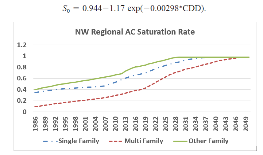
In addition to direct impacts through increased temperature and changed precipitation patterns, there are also indirect actions that impact loads. Increases in acquisition and use of Air-Conditioning (AC) in the residential sector is a case in point. Although most residences in NW states did not have or use AC (because of short and mild summer season), a recent Residential Building Stock Assessment (RBSA) survey found a significant jump in the number of homes with mechanical cooling. Between RBSA I (2010) and RBSA II (2018) the percent of single-family homes with mechanical cooling jumped from 36% to 63%.
This level of increase in AC saturation rate has already occurred. To project a forecast of AC saturation rates in the future we need additional information as to how consumers’ decisions to purchase AC are influenced by increases in temperature. We used the structural relationship developed by, “D.J. Sailor, A.A. Pavlova (2003)” measuring AC saturation rate (S) as a function of cooling requirement (CDD). Results from the relationship below was then compared to RBSA findings. After a simple forced calibration to RBSA finding, we created a forecast of AC saturation rate for 2019-2049. Using state level CDD data for 1985-2017 we calculated state level AC saturation rate and compared it to RBSA II survey findings. Overall survey results were 10% above the results from the equation. A modified equation was then used to forecast AC saturation rate for the future time period. Future AC saturation rates were capped at 98%. The graph below shows regional saturation rates for the NW. Manufactured homes are labeled as Other Family in this graph.
Indirect effects of Climate Change: Increase in migration
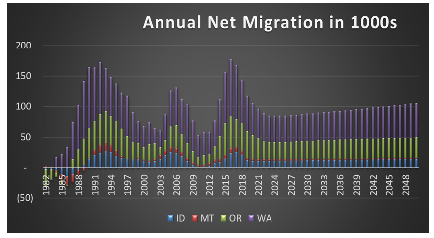
Change in temperatures resulting from climate change not only will increase demand for cooling and reduce demand for heating, it can impact other aspects of the economy and demographics of the region. Existing literature shows populations that are under economic stress and, given the opportunity, will migrate to areas with better economic opportunity. Existing studies also indicate that the Northwest may be in a better competitive position compared to the Mid-west or the South. This competitive advantage is expected to lead to changes in net migration into the region. This indirect or secondary impact will be felt gradually. A companion report discussing migration impact of climate change is available here.
Patterns of in- or out-migration are indicative of the economic health of a region. Graphs below track the net-migration into the Northwest. On average, between 1982-2018, 94,000 people migrated annually to the Northwest. Over the next 30 years (by 2050), we are estimating a net increase migration that would grow the regional population by an additional 1.3 million people, as shown in the figure and table below:
Additional Population Growth Estimates to 2050
| Impact in 2050 | Washington | Oregon | Idaho | Montana | Region |
| Population in 2017 | 7,420,309 | 4,149,843 | 1,721,235 | 1,051,812 | 14,343,199 |
| Forecast Population in 2050 | 9,461,199 | 5,110,406 | 2,435,690 | 1,159,014 | 18,166,309 |
| Additional Migration | 864,981 | 338,895 | 157,957 | (35,478) | 1,326,355 |
| Total 2050 Population | 10,326,180 | 5,449,301 | 2,593,647 | 1,123,536 | 19,492,664 |
| Additional Growth | 9.1% | 6.6% | 6.5% | -3.1% | 7.3% |
| Total Growth from 2017 to 2050 | 39% | 31% | 51% | 7% | 36% |
Another secondary impact of increased net migration is increased demand for resources. This could cause an increase in the cost of housing and lower per capita income. Which would shift more new residential construction from single to multifamily. At the start of the 2021 plan, single family residences make up about 70% of new residential construction with multifamily construction making up 20%. To incorporate impacts of increased population and increased housing cost, we have lowered the market share for new single-family units over the next 30 years by 20% and increased multifamily units by 20%. The overall change (over the next 30 years) shows a shift of about 218,000 new homes from Single-family to Multi-family units.
Change in Market Share and cumulative Number of Additions by Residence Type (by 2050)
| Current Trend | With Climate Change | Current Trend Cumulative BY 2050 | With Climate Change Cumulative BY 2050 | Delta Cumulative by 2050 | |
| Market Share | Market Share | Number (1000) | Number (1000) | Number (1000) | |
| Single Family | 70% | 50% | 763 | 545 | (218) |
| Multi-Family | 20% | 40% | 218 | 436 | 218 |
| Other/MH | 10% | 10% | 109 | 109 | 0 |
What are the economic impacts of this increase in population?
How much more commercial floorspace would be needed? How would the industries in the region react to this increase in population? Would manufacturing output in the region increase or decrease and by how much? To quantify impacts of the expected increase in population, we used the concept of elasticity, relating the percent change in population to the percent change in sector level output.
An example: What is the elasticity of agricultural output relative to population? If population changes by one percent, how much does agricultural output change? The ratio of percent change in one variable to the percent change in the second variable measures the elasticity of response between the two variables.
Beginning with the equation:
log(agricultural output)=A*log(population) + constant + error term
The term on the right-hand side of the structural equation capture the percent change in population, and the term on the left-hand side represent percent change in Agricultural output, so coefficient of population measures the elasticity of response in agricultural output when population change. Suppose we obtain the estimates
log (Agricultural output)=0.45*logpopulation+2.1
Coefficient 0.45 means that for every 1% change in population, agricultural output increases by 0.45%.
To calculate the elasticity (or change) in a particular variable due to a change in population requires having a dependable set of data for both variables. Typically, historic values for both variables are used to estimate elasticities.
In our case we are using both historic and future values for population and either industrial outputs or commercial floorspace requirements. The reason we are using future values is to recognize that industrial output in the region may be changing and we want to capture these structural changes. This is in lieu of using an integrated macro-economic model. We are using the state level forecast of outputs from manufacturing sectors from Global Insight and relating it to forecasted population.
The mechanics of estimating the elasticities is straight forward. Take historic and forecast of industrial output (adjusted for inflation) and relate it to historic and forecast of population. We do this at the state and industry level. In our case history starts in 1985 and goes to 2050. We tested for the non-stationary nature of the two variables but given that our application is not a traditional forecast, we felt that for practical reasons creating a stationary set of variables is not needed. We did correct for any autocorrelation in the structure of the models. When current value of an independent variable depends on value of same variable in previous periods, then an autocorrelation in the structure exist. Without correcting for autocorrelation, estimated coefficients are not stable and not reliable for forecasting future values of the dependent variable. We estimated correlation values between the dependent variable and population using 188 separate state level equations. The table below shows percent change in the parameters listed because of a one percent change in population.
| Sector | Oregon | Washington | Idaho | Montana |
| Residences | 0.84 | 0.91 | 0.85 | 1.0 |
| Commercial sectors combined | 0.56 | 0.91 | 0.62 | 0.68 |
| Agriculture | 0.40 | 0.45 | 0.64 | 0.23 |