


Transforming Outputs from Load Forecast Model for Input into Redeveloped GENESYS
This section contains descriptions of the R-script that transforms outputs from the Council’s load forecast model and incorporates hourly shapes for energy conservation to become input data for the redeveloped GENESYS model.
Among the many inputs into the Council’s load forecast model are forecasted temperature data for 2020 to 2049 from climate scenarios produced by the River Management Joint Operating Committee (RMJOC, see Summary of Climate Change Scenarios write-up for more details). The load forecast model produces two types of outputs: the weather-normalized loads and the temperature-sensitive multipliers (Method to Forecast Climate Change Loads for more details). Energy efficiency hourly capacity factors and average energy efficiency saving could also be incorporated with the outputs to calculate the Northwest regional load for resource adequacy studies. The R-script transforms and formats these data into inputs for the redeveloped GENESYS model.
The Weather-Normalized Loads
The load model has as inputs the forecasted regional temperatures from three selected RMJOC climate scenarios, A, C and G, for the 30 years from 2020 to 2049 (see climate change scenarios selection write-up for more details). Then from the forecasted temperatures for a climate scenario, monthly cooling-degree-days (CDDs) and heating-degree days (HDDs) are calculated and used to derive the monthly weather-normalized Northwest regional loads for a selected year (e.g., 2025, 2031). The average of the 30 years of forecasted temperatures (as determined within the load model) is then used to transform the monthly weather-normalized loads into the hourly weather-normalized loads for the selected year.
To simulate operations of the Northwest power system for an operating year, three levels of hourly weather-normalized loads are calculated: the high, medium and low load forecasts. For convenience for the Power Plan, the weather-normalized loads were calculated for all 30 years, from 2020 to 2049. As an example, a portion of the medium forecast weather-normalized loads for the RMJOC climate scenario G is presented in Figure 1.
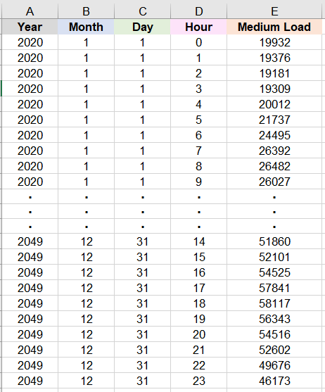
Figure 1: An example medium forecast weather-normalized load for climate scenario G for 2020 to 2049.
In Figure 1, columns A to D list the operating years, months, days and hours for the medium weather-normalized load forecast in column E, in units of MW. For convenience, leap days are not included in columns A to D. Thus, there are 262,800 rows of data for the 30 years of hourly loads.
The medium weather-normalized load forecast for a particular operating year is then obtained from filtering the year, month and day columns in Figure 1. For example, for operating year 2031, which starts on 10/1/2030 and ends on 9/30/2031, the 8,760 rows of hourly loads filtered from Figure 1 are presented in Figure 2.
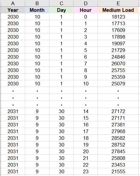
Figure 2: Filtered loads from Figure 1 for operating year 2031.
The Temperature-Sensitive Multipliers
In addition to weather-normalized loads, the load model also produces temperature-sensitive multipliers (TSMs) for each of the 30 temperature-years, from 2020 to 2049. The TSMs are calculated from the deviations between the average temperatures and forecasted temperatures for a particular temperature-year. Then TSMs for a particular temperature-year are used to multiply the weather-normalized loads to obtain loads that are under the influence of temperatures of that same temperature-year. A portion of an example TSM output for climate scenario G, after formatted by the R-script, is presented in Figure 3.
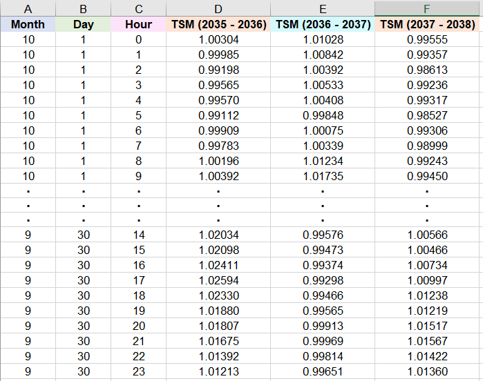
Figure 3: Temperature-sensitive multipliers (TSMs) for climate scenario G for temperature-years 2035 to 2038.
In Figure 3, columns A to C list the 8,760 rows of months, days and hours for the TSM values in columns D to F. Both the weather-normalized loads and TSMs in Figures 1 and 2 respectively are derived using temperature data from climate scenario G. Furthermore, as an example, in column D, the TSMs values for months 10 to 12 (listed in column A) are derived using forecasted temperatures for 2035, while the values for months 1 to 9 are derived using forecasted temperatures for 2036. Similarly, in column F, for months 10 to 12, the TSMs are calculated using forecasted temperatures for 2037, while TSM values for months 1 to 9 are calculated using forecasted temperatures for 2038. Due to space limitation, only the 3 sets (instead of 30) of TSMs are presented in Figure 3.
Therefore, for climate scenario G, the Northwest regional loads for operating year 2031 under the influence of temperatures from month 10, 2037 to month 9, 2038, are calculated by multiplying the load values in column E in Figure 2 to the corresponding TSM values in column F in Figure 3. The calculations are discussed in detail in a later section.
Energy Efficiency Capacity Factors
For operating year 2031, example hourly capacity factors produced by a representative energy efficiency load profile (the profile is calculated by a weighted average of profiles from low-cost energy efficiency measures) is presented in Figure 4.
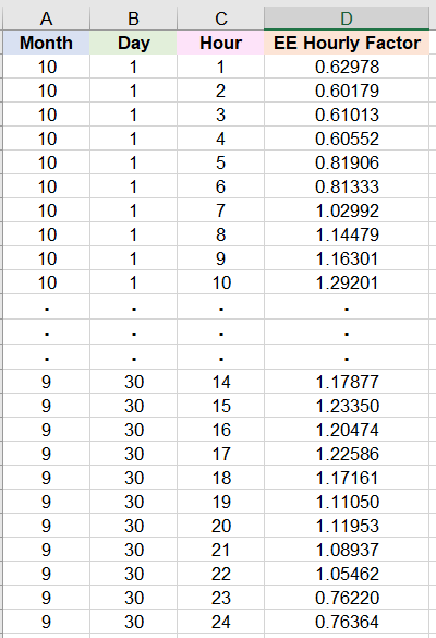
Figure 4: Example energy efficiency hourly capacity factors.
In Figure 4, columns A to C list the 8,760 rows of months, days and hours for the energy efficiency hourly capacity factors. For resource adequacy studies, the energy efficiency savings, obtained by multiplying the hourly capacity factors with an average energy efficiency saving (in units of aMW) chosen for the studies, are subtracted from the weather-sensitive loads. The next section shows an example calculation.
Example Calculations of the Northwest Regional Load
This section shows example calculations of the Northwest regional load from weather-normalized loads, temperature-sensitive multipliers and energy efficiency savings. More specifically, the regional load is calculated for operating-year 2031 under the influence of the 2037 to 2038 temperatures with 1,200 aMW of average energy efficiency saving.
For the regional load calculations, relevant data in Figures 2, 3 and 4 are merged which result in Figure 5.
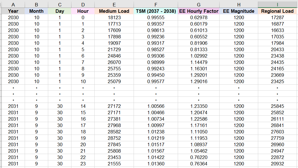
Figure 5: Relevant data in Figures 2, 3 and 4 are merged. In addition, column H contains a 1,200 aMW energy efficiency saving.
In Figure 5, columns A to D list the years, months, days and hours of operating year 2031. Then column E contains the medium forecast weather-normalized loads. After that, column F lists the TSM values derived from temperatures for 2037 (for months 10 to 12) and 2038 (for months 1 to 9). Finally, columns G and H contain energy efficiency hourly capacity factors and an average energy efficiency saving, respectively.
Let represents the weather-normalized load for operating-year 2031. Then let
represents the temperature-sensitive multipliers for the 2037 and 2038 temperature-years. Furthermore, let
and
represent the energy efficiency hourly capacity factors and average energy efficiency saving (1,200 aMW) respectively. Thus, the regional load for operating-year 2031 under the influence of the 2037 to 2038 temperatures with 1,200 aMW of energy efficiency savings subtracted is calculated as
which results in the values listed in column I. For example, on the first row in Figure 5 where calendar year = 2030, month = 10, day = 1 and hour = 0, ,
,
, and
. Then
on the first row of column I. For simplicity, Direct-Service Industry (DSI) loads are not included in the calculations.
Transforming the Northwest Regional Loads into Inputs for the Redeveloped GENESYS
This section discusses transformation of the Northwest regional loads, presented in column I in Figure 5, into loads for the 17 Northwest balancing areas modeled in the redeveloped GENESYS. The names for the 17 Northwest balancing areas used in the model are listed in Figure 6.
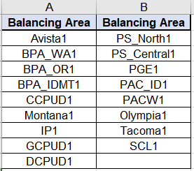
Figure 6: Names for the 17 Northwest balancing areas used in the redeveloped GENESYS model.
In Figure 6, the names Avista, Montana, Olympia and Tacoma represent obvious balancing areas. In addition, BPA_WA, BPA_OR and BPA_IDMT represent the three areas associated with Bonneville Power in Washington, Oregon, and Idaho – Montana respectively. Furthermore, CCPUD, GCPUD and DCPUD represent the public utility districts of Chelan County, Grant County and Douglas County respectively. Moreover, IP, PGE and SCL represent Idaho Power, Portland General Electric and Seattle City Light respectively. Finally, PS_North, PS_Central and PAC_ID and PACW represent two balancing areas for Puget Sound Energy and PacifiCorp respectively. A detailed map for the 17 balancing areas could be viewed using the web-interface for the redeveloped GENESYS model.
Each of the balancing area in Figure 6 has its hourly fractional share of the Northwest regional loads listed in Column I in Figure 5. These hourly fractional shares are average of 2012-2019 observed BA load as a fraction of regional load. A portion of their hourly shares are presented in Figure 7.
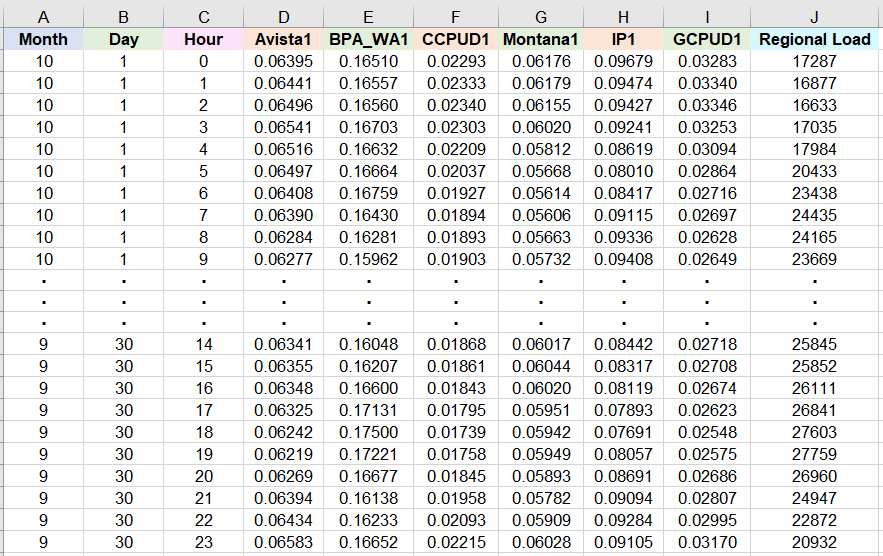
Figure 7: Hourly fractional shares of the Northwest regional load for several balancing areas modeled in the redeveloped GENESYS. For convenience, the Northwest regional load is also printed in column J.
In Figure 7, due to space limitations, only data for 6 of the 17 balancing areas are presented. Columns A to C list the 8,760 rows of months, days and hours for the fractional share data of the 6 balancing areas in columns D to I. For example, for month = 10, day = 1 and hour = 0 on the first row, the Avista share of the Northwest regional load (in column D) is 0.06395 or approximately 6.4%. For CCPUD and GCPUD, their shares (in columns F and I respectively) are 0.02293 and 0.03283, or approximately 2.3% and 3.3% respectively. Finally, for convenience, column J contains the Northwest regional load copied from column I in Figure 5.
The loads for the 6 balancing areas presented in Figure 7 are obtained by multiplying their respective fractional shares to the Northwest regional load in column J. The results are presented in Figure 8.
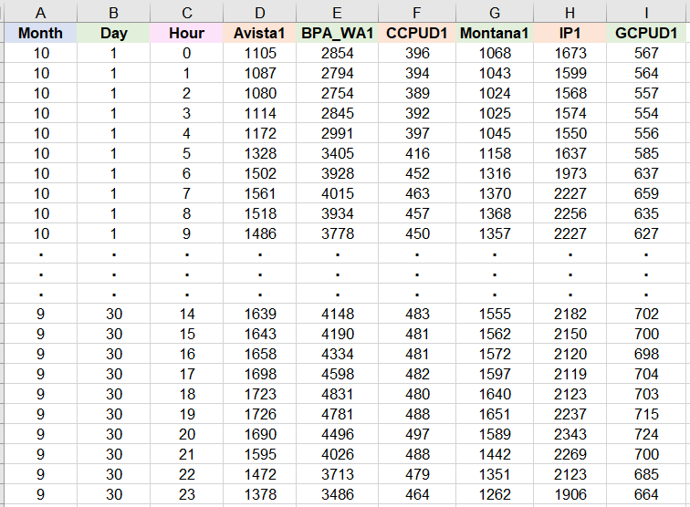
Figure 8: Hourly loads for 6 balancing areas presented in Figure 7.
In Figure 8, columns A to C list the 8,760 rows of months, days and hours for the load values of the 6 balancing areas in columns D to I. For example, on the first row, for month = 10, day = 1 and hour = 0, the Avista load of 1,105 MW is calculated by (0.06395)×(17,287 MW) from the first row of columns D and J respectively in Figure 7. (Because the values (0.06395) and (17,287 MW) had been rounded to five significant figures, their product is actually 1,105.5 MW. With one more significant figure for the two values, their product would be 1,105.4 MW which rounds to 1,105 MW as presented in Figure 8.)
In summary, a part of the R-script combines the algorithms described in previous sections that incorporate weather-normalized loads, temperature-sensitive multipliers and energy efficiency hourly capacity factors and average energy efficiency saving to calculate the regional loads. With the regional loads, another part of the R-script then uses the fractional shares for the 17 balancing areas to calculate loads for each of the balancing area.
For the example data discussed and presented previously, the R-script calculates hourly loads, as shown in Figure 8, for the 6 balancing areas for the 2031 operating year under the influence of the forecasted 2037 and 2038 temperatures of climate scenario G with 1,200 aMW of energy efficiency saving. However, for resource adequacy study for the same 2031 operating year, the R-script would calculate loads for all 17 balancing areas using about a decade of forecasted temperatures, from 2029 to 2039, for each of the three RMJOC climate scenarios, A, C and G. In addition, the R-script also transforms the Month, Day and Hour columns in Figure 8 into weekly formatted columns for inputs into the redeveloped GENESYS model.