


For the 2021 Power Plan, the Council decided to use climate data developed by the River Management Joint Operating Committee (RMJOC). A comprehensive report on the RMJOC climate data is available in RMJOC report I. In the report, RMJOC staff selected 19 climate scenarios for reservoir regulation studies in order to model and analyze climate impacts on hydro power, flood risk management, water supply, ecosystem and biological operations, among other topics of interest. Results of the hydro-regulation studies are published in RMJOC report II. To ensure a timely completion of the Power Plan, the Council selected a representative subset of the 19 RMJOC climate scenarios for study. The following sections contain the Council’s methodology for selecting scenario in the context of power system adequacy, and an analysis of the selected scenarios. These sections also reference the RMJOC climate scenarios from Summary of the RMJOC Climate Scenarios.
Variables to Select Subset of Climate Scenarios
For the 2021 Power Plan, the Council, to varying degrees, has incorporated climate scenario wind and historical solar generation along with the RMJOC climate temperatures and hydro-related data in all of its analytical tools, including the classic GENESYS and redeveloped GENESYS models that perform power system adequacy studies. However, the 19 RMJOC climate scenarios (listed in Table 3 in Summary of the RMJOC Climate Scenarios) are still too many to run studies and analyze results to enable the power plan to be completed in a timely manner. Thus, in the context of power system adequacy, the Council decided to select a small subset of the 19 scenarios to represent their range of uncertainty in summer and winter hydro generation, and in summer and winter regional load. For example, for either season, a high adequacy range is likely to be achieved under high hydro generation and low loads, while conversely a low adequacy range is likely to occur for low hydro generation and high loads. And intermediate levels of adequacy are likely to be realized under other combinations of hydro generation and loads.
Monthly hydro generation for all hydro-projects is calculated by HDYSIM, the hydro regulation model inside of the classic GENESYS model, in which climate data from the 19 RMJOC scenarios have been incorporated. For scenario selection based on the aggregate hydro generation (more details in a later section), classic GENESYS was run for each scenario in a similar way that it is run for the Council’s yearly Resource Adequacy Assessment. For those studies, the operation of the northwest power system is modeled for a future operating year under varying hydro conditions and loads. For the scenario selection studies, the future operating year is 2028, and for each scenario, the hydro conditions are the 30 years of forecasted streamflows and hydro-regulation related data from 2020 to 2049. However, unlike the usual adequacy assessment studies, all other classic GENESYS inputs (that could affect hydro generation) are held constant in order to isolate differences in hydro generation due to streamflows across the 19 climate scenarios. More specifically, the same one-year set of hourly loads and historical hourly wind and solar capacity factors were used for all 19 climate scenarios. The hourly loads are calculated from observed temperatures over a historical time period and thus do not include any effects from projected climate scenario temperatures. Furthermore, the random thermal forced outages normally activated for adequacy assessment studies have been turned off.
For scenario selection based on load, surrogate variables were used due to the significant time and effort that would be required to calculate hourly loads over 30 years for all 19 scenarios. Instead, scenario selection was based on more easily calculated quantities: monthly heating degree-days (HDDs) and cooling degree-days (CDDs). The winter HDDs and summer CDDs are used as simple proxies for winter and summer loads, respectively. Details of this selection process are presented in a later section.
Thus, by selecting a few scenarios that are representative of the range of summer and winter hydro generation and the range of summer CDDs and winter HDDs of the ensemble of 19 RMJOC climate scenarios, the Council was able to develop this plan in a timely fashion.
The Selection Methodology for Climate Scenarios
In this section, an algorithm is developed to analyze and rank the four monthly variables, summer and winter hydro generation and summer CDDs and winter HDDs, for the 19 climate scenarios over the 30-years from 2020 to 2049. Then, based on the rankings and other considerations, scenarios are selected to represent the high and low levels for the four variables.
A priori, there could potentially be eight scenarios selected to represent high and low levels of the four variables as illustrated in Table 1 below.
Table 1: The eight potential scenarios, S1, …, S8, selected to represent high and low levels of the four variables: summer and winter hydro generation, and summer CDDs and winter HDDs.
| Level | Summer Hydro Generation | Winter Hydro Generation | Summer CDDs | Winter HDDs |
| High | S1 | S2 | S3 | S4 |
| Low | S5 | S6 | S7 | S8 |
However, eight scenarios will still require too much time and resources to perform simulations and analyses for the Power Plan. Thus, instead of always selecting the scenario ranked first by the algorithm, when appropriate, as an approximation, the Council selected scenarios that were nearby second choices, if they are also able represent more than one slot in Table 1, and thus reducing the total number of selected scenarios.
Scenario Selection Based on Summer and Winter Hydro Generation
This section begins with an analysis of monthly hydro generation produced by the HYDSIM model within classic GENESYS. The months of interest are December, January and February, representing winter, and June, July and August, representing summer.
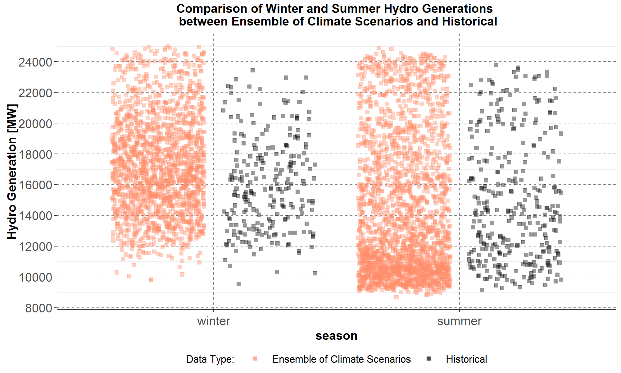
Figure 1 presents a comparison of winter and summer hydro generations between the ensemble of the 19 climate scenarios and the historical 80 water-years (1929 – 2008). The ensemble is plotted in orange while the historical is plotted in black, with winter generations on the left and summer generations on the right. The magnitudes of the average monthly generations are along the y-axis and labeled as [MW]. For each season, the ensemble generation contains (3 months) x (30 future water-years) x (19 scenarios) = 1,710 data points, whereas the historical generation has (3 months) x (80 historical water-years) = 240 data points. The plots in Figure 1 are known as jitter plots where the data are spread out in the horizontal direction so that fewer of them are plotted on top of one another and thus enable their distribution along the vertical direction to be more easily observed.
The plots in Figure 1 suggest that, compared to the corresponding seasonal historical generation, the ensemble, on average, has higher generation for winter and lower generation for summer.
Figure 1: Comparisons of winter generations (on the left) and summer generations (on the right), between the ensemble of 19 climate scenarios (in orange) and historical (in black). The magnitudes of the hydro generations are along the y-axis
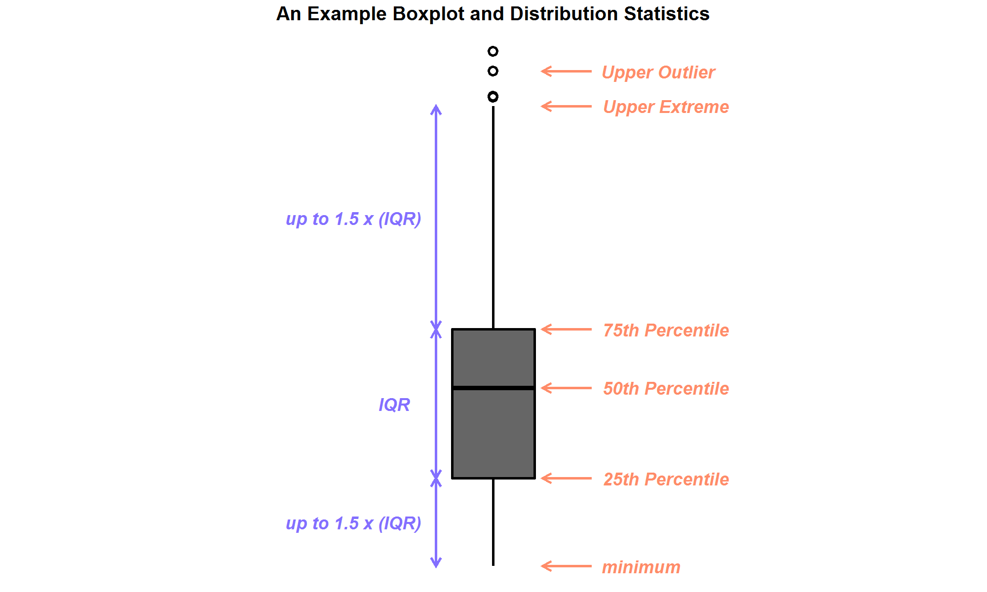
In contrast to the jitter plot in Figure 1, the box-and-whiskers plot, or simply the boxplot, as illustrated in Figure 2, allows for quantitative comparisons of distributional statistics such as the 25th, 50th (the median) and 75th percentiles. The grey box in Figure 2, which starts from the 25th percentile and ends at the 75th percentile, contains the central 50% of the population of the distribution. The length of the box is defined as the inter-quartile-range (IQR) and is used to delineate outliers (if any): those data that lie beyond one-and-a-half times the IQR from the box.
Figure 2: An example box-and-whiskers plot or boxplot, with upper outliers shown
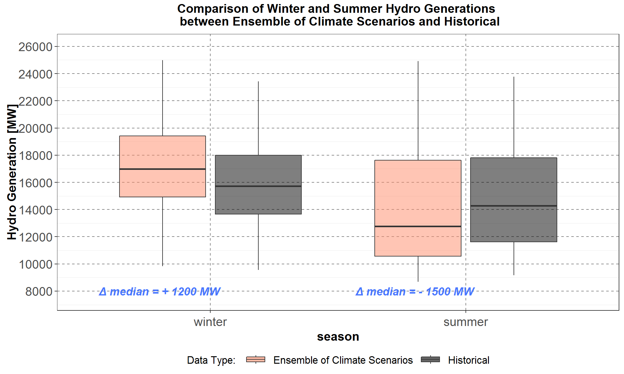
Thus, Figure 3 presents the same data as in Figure 1 but in terms of boxplots. For example, from comparing medians, which is the black line inside each box, the plots show that the climate ensemble is 1,200 MW higher than historical for winter, and conversely 1,500 MW lower than historical for summer. Thus, under the effects of potential future climates, on average, there should be higher winter and lower summer hydro generation.
Figure 3: Comparisons of winter generations (on the left) and summer generations (on the right), between the ensemble of 19 climate scenarios (in orange) and historical (in black).
The magnitudes of the hydro generations are along the y-axis. Compared to median historical generations, the ensemble median is 1,200 MW higher for winter but 1,500 MW lower for summer
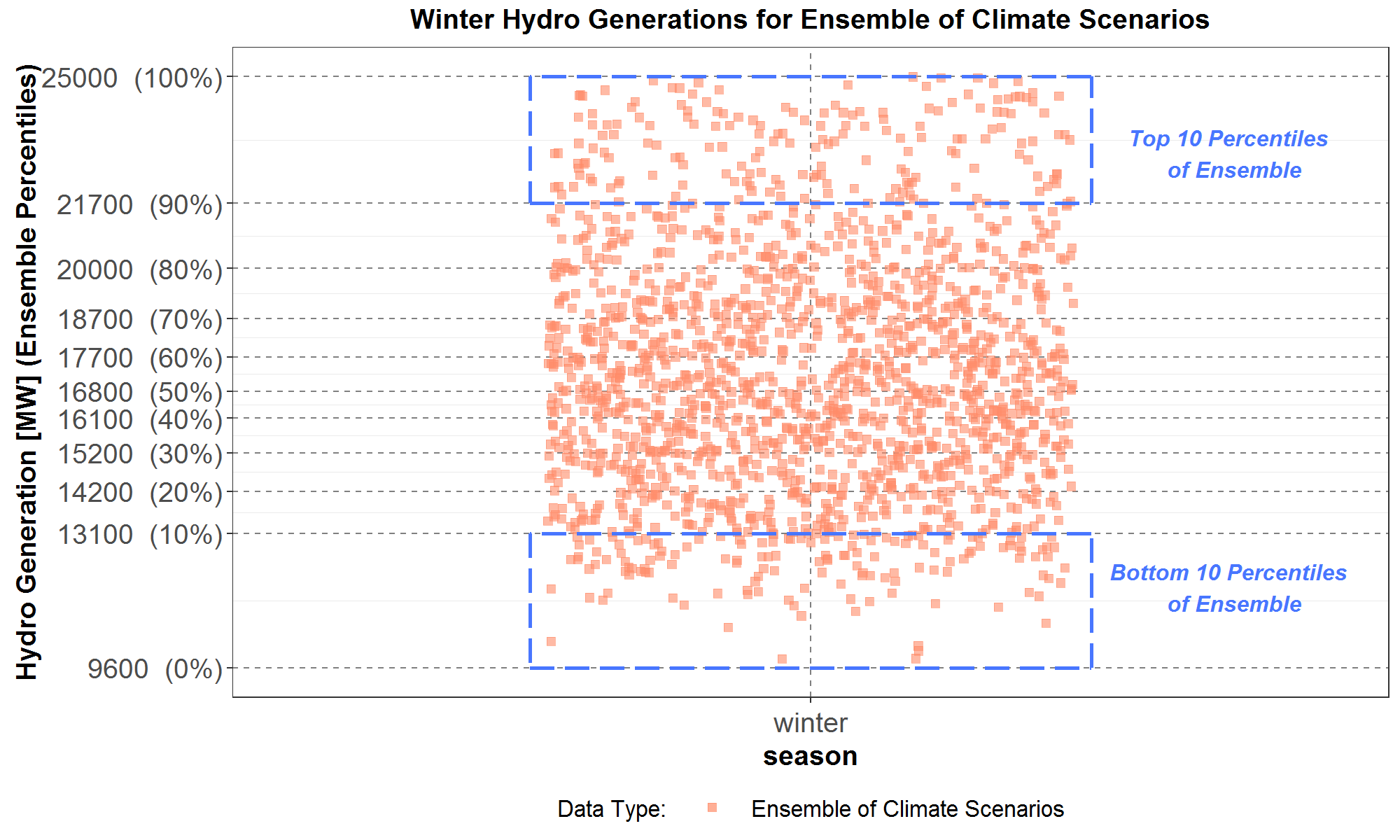
Next in Figure 4, the ensemble winter generation in Figure 1 is magnified and an algorithm is developed to select scenarios that represent its high and low levels. The ensemble winter generation has been divided into 10 equal-population slices by the y-axis grid lines and the ensemble deciles are printed inside parentheses along the y-axis. For example, the bottom-10 percentiles are between 9,600 MW and 13,100 MW (rounded to nearest 100 MW) and delineated by the lower blue dashed box, while the top-10 percentiles are between 21,700 MW and 25,000 MW and delineated by the upper blue dashed box. The algorithm then selects the scenario with the highest population in the bottom-10 percentiles to represent low ensemble hydro generation. Similarly, the algorithm selects the scenario with the highest population in the top-10 percentiles to represent high ensemble hydro generation.
Figure 4: The ensemble winter generation divided into 10 equal-population slices, or deciles. The deciles are divided by the y-axis grid lines and printed inside parentheses (rounded to nearest 100) along the y-axis.
The bottom-10 and top-10 ensemble percentiles are delineated respectively by the lower and upper blue dashed boxes.
The selection algorithm is demonstrated by breaking up the ensemble winter generation in Figure 4 into its components of 19 scenarios, which are plotted in Figure 5. The 19 scenarios are listed by scenario indices along the x-axis, from A to S, according to Table 3 in Summary of the RMJOC Climate Scenarios. Once again, the ensemble deciles are inside parentheses along the y-axis. The algorithm selects the scenario with the most data points between the 0% and the 10% y-axis grid lines, and the scenario with the most data points between the 90% and the 100% grid lines. For comparison, the historical winter generation is also plotted as scenario T.
Figure 5: Winter generations of the 19 climate scenarios with indices from A to S according to Table 3 in Summary of the RMJOC Climate Scenarios.
The historical winter generations are also plotted and have index T. The y-axis grid lines are deciles of the ensemble winter generation
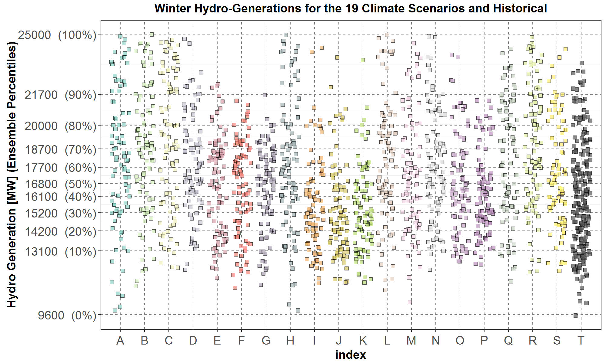
Results of the population counts for each scenario in the bottom-10 and top-10 ensemble percentiles in Figure 5 are listed in Table 2 below.
Table 2: Population of the 19 climate scenarios within the bottom-10 and top-10 ensemble percentiles for winter generation.
| Scenario Index | Population in the Bottom-10 Ensemble Percentiles | Population in the Top-10 Ensemble Percentiles | Scenario Index | Population in the Bottom-10 Ensemble Percentiles | Population in the Top-10 Ensemble Percentiles |
| A | 22 | 8 | K | 5 | 13 |
| B | 14 | 6 | L | 19 | 12 |
| C | 22 | 7 | M | 14 | 13 |
| D | 8 | 14 | N | 9 | 13 |
| E | 11 | 12 | O | 7 | 10 |
| F | 11 | 15 | P | 4 | 16 |
| G | 12 | 20 | Q | 8 | 9 |
| H | 11 | 10 | R | 15 | 10 |
| I | 6 | 13 | S | 17 | 15 |
| J | 13 | 11 |
According to Table 2, scenario J has the highest population in the bottom-10 ensemble percentiles, at 23; and scenario C has the highest population in the top-10 ensemble percentiles, at 30. Therefore, J and C are selected to represent the low and high ensemble winter hydro generation, respectively.
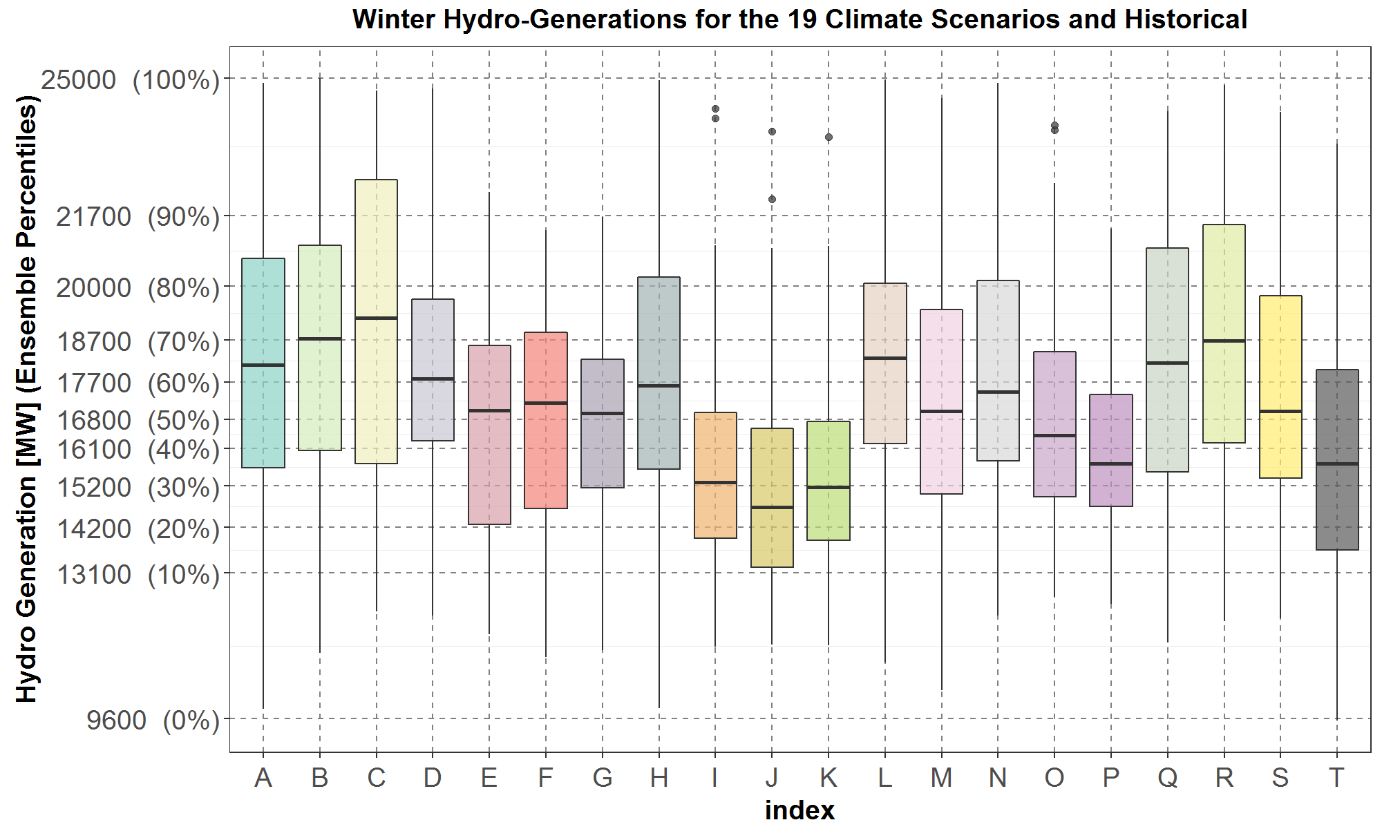
The same winter generation data in Figure 5 are also presented in boxplots in Figure 6. It shows that on average, only scenarios I, J and K among the 19 RMJOC scenarios have lower winter hydro generations than historical (scenario T) since their medians, 75th percentiles and upper whiskers are lower than historical. In addition, according to Table 2, scenarios I, J and K have the three highest populations in the bottom-10 ensemble percentiles. However, hydro generation is dependent on streamflow and from Table 3 in Summary of the RMJOC Climate Scenarios, it turns out that streamflow and other climate data for all three scenarios are derived from the same GFDL-ESM2M Global Climate Model (GCM). Furthermore, according to Figures 48 and 49 in RMJOC report I, that GCM produces streamflows that tend not to exhibit the general climate seasonal-shift characteristics of higher average fall and winter flows, earlier peak spring runoff, and longer periods of low summer flows. Since the Council wants to explore the risk of these seasonally shifted climate streamflows, then the three GFDL-ESM2M derived scenarios, I, J and K, are removed from the selection process for winter hydro generation. It then follows that they are also excluded from subsequent selections for summer hydro generation, winter HDDs and summer CDDs as well. However, it is important to determine if excluding scenarios I, J and K from being selected would introduce a significant bias in the finalized set of selected scenarios. This issue is analyzed in a subsequent section. Finally, according to Table 2, scenario F has the highest population, at 12, after I, J and K have been excluded. Thus, F is selected to represent the low ensemble winter hydro generation.
It is also interesting to note from Figure 5 that the distributions for F and G are very similar, which should not be too surprising since according to Table 3 in Summary of the RMJOC Climate Scenarios, they have the same GCM (CNRM-CM5) with the same downscaling method (MACA), and differ only on the hydrological models used. Furthermore, according to Table 2, F has just one more population than G in the bottom-10 ensemble percentiles.
After the considerations mentioned above, scenarios C and F are selected to represent the high and low ensemble winter hydro generations, respectively.
Figure 6: Winter generations of the 19 climate scenarios with indices from A to S according to Table 3 in Summary of the RMJOC Climate Scenarios. The historical winter generations are also plotted and have index T. The y-axis grid lines are deciles of the ensemble winter generation. The medians, 75th percentiles and upper whiskers for scenarios I, J and K are lower than those of the historical
After selecting scenarios C and F to approximately represent the full range of the ensemble winter generation (to be analyzed in a subsequent section), the algorithm is next applied to the ensemble summer generation to select its representative scenarios. Summer generations for the 19 scenarios are plotted in Figure 7. Similar to Figure 5, each of the 19 scenarios are listed by its index along the x-axis according to Table 3 in Summary of the RMJOC Climate Scenarios, and the historical summer generation is plotted as scenario T. The ensemble summer generation deciles are inside parentheses along the y-axis. Among the remaining scenarios after excluding I, J and K, the algorithm selects the scenario with the most data points between the 0% and the 10% grid lines, and the scenario with the most data points between the 90% and the 100% grid lines.
Figure 7: Summer generations of the 19 climate scenarios with indices from A to S according to Table 3 in Summary of the RMJOC Climate Scenarios. The historical summer generations are also plotted and have index T. The y-axis grid lines are deciles of the ensemble summer generation
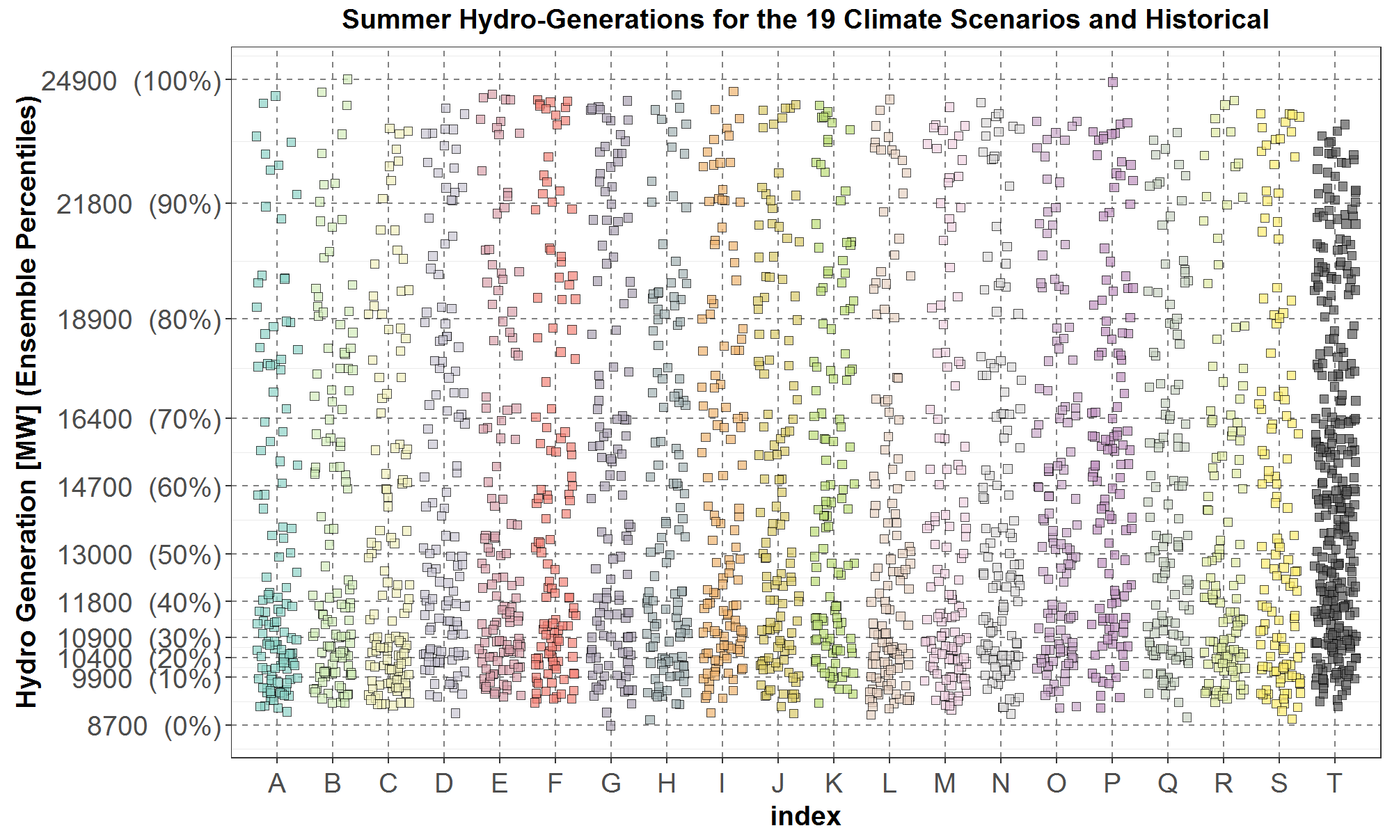
Table 3 below lists the population count for each scenario in the bottom-10 and top-10 ensemble percentiles in Figure 7.
Table 3: Population of the 19 climate scenarios within the bottom-10 and top-10 ensemble percentiles for summer generation.
| Scenario Index | Population in the Bottom-10 Ensemble Percentiles | Population in the Top-10 Ensemble Percentiles | Scenario Index | Population in the Bottom-10 Ensemble Percentiles | Population in the Top-10 Ensemble Percentiles |
| A | 22 | 8 | K | 5 | 13 |
| B | 14 | 6 | L | 19 | 12 |
| C | 22 | 7 | M | 14 | 13 |
| D | 8 | 14 | N | 9 | 13 |
| E | 11 | 12 | O | 7 | 10 |
| F | 11 | 15 | P | 4 | 16 |
| G | 12 | 20 | Q | 8 | 9 |
| H | 11 | 10 | R | 15 | 10 |
| I | 6 | 13 | S | 17 | 15 |
| J | 13 | 11 |
According to Table 3, both scenarios A and C have the highest population in the bottom-10 ensemble percentiles, at 22. It would be desirable to select both A and C for completeness, but as mentioned previously, there is only enough time and resources to study and analyze a few scenarios for the Power Plan. Therefore, since C has already been selected to represent high ensemble winter generation, then C is also selected to represent low ensemble summer generation to keep the total number of selected scenarios small.
Also, from Table 3, scenario G has the highest population in the top-10 ensemble percentiles, at 20. Therefore, G is selected to represent high ensemble summer generation.
Thus, scenarios C, F and G have been selected to represent high and low ensemble winter and summer generations. However, in the next section, it is likely that other scenarios will be selected to represent high and low ensemble winter HDDs and summer CDDs. Since the Council is also concerned about the computational burden of running the newly redeveloped GENESYS model, limiting the total scenarios to three or four scenarios rather than more would allow for substantial reduction in the computational cost of running the new model. Therefore, it will be prudent to check if one of the three scenarios, C, F and G could be eliminated. Fortunately, as discussed previously, for winter generations, G is very similar to F in Figure 5, and according to Table 2, G has just one fewer population than F in the bottom-10 ensemble percentiles for winter generation. Thus, as an approximation, G, instead of F, is selected to represent low ensemble winter generation. The reason for keeping G and dropping F becomes clear in the next section.
Therefore, after excluding scenarios I, J and K, the algorithm selected C to represent both high ensemble winter and low ensemble summer generation, and conversely selected G to represent both low ensemble winter (as an approximation) and high ensemble summer generation. The two selected scenarios, C and G, occupy the four slots for hydro generation in Table 1.
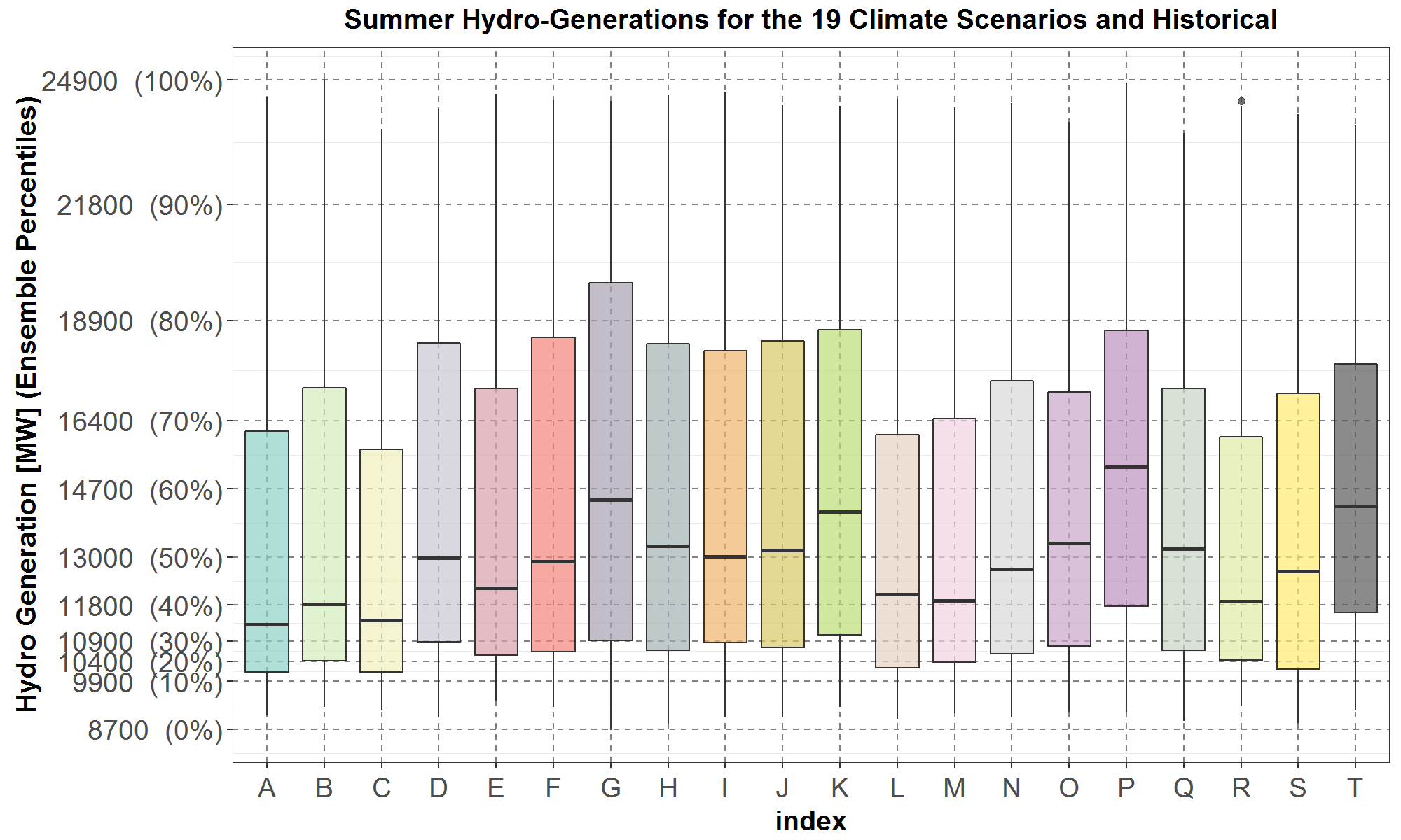
For completeness, Figure 8 presents the same data in Figure 7 in boxplots. It shows that most scenarios have lower medians than historical (scenario T), and all scenarios have lower 25th percentiles than historical.
Figure 8: Summer generations of the 19 climate scenarios with indices from A to S according to Table 3 in Summary of the RMJOC Climate Scenarios.
The historical summer generations are also plotted and have index T. The y-axis grid lines are deciles of the ensemble summer generation
Scenario Selection Based on Monthly Cooling Degree-Days and Heating Degree-Days
Unlike the northwest hydro system generation presented previously, which is an output of the classic GENESYS model, the regional monthly cooling degree-days (CDDs) and heating degree-days (HDDs) are directly calculated from regional temperatures. The regional temperature T is not the temperature at any specific location, but a weighted sum of temperatures of four northwest cities, Seattle, Portland, Spokane and Boise, and a constant term and is expressed as follows:
T = a*TSeattle+ b*TPortland+ c*TSpokane+ d*TBoise+ k (1)
where coefficients a , b , c , d and constant k vary by months as indicated in Table 4 below.
Table 4: Monthly coefficients a , b , c , d and constant term k for transforming temperatures for Seattle, Portland, Spokane and Boise to the regional temperature
| Month | a | b | c | d | k |
| 1 | 0.492 | 0.258 | 0.219 | 0.062 | -2.544 |
| 2 | 0.492 | 0.258 | 0.219 | 0.062 | -2.544 |
| 3 | 0.492 | 0.258 | 0.219 | 0.062 | -2.544 |
| 4 | 0.492 | 0.258 | 0.219 | 0.062 | -2.544 |
| 5 | 0.352 | 0.192 | 0.203 | 0.150 | 6.542 |
| 6 | 0.352 | 0.192 | 0.203 | 0.150 | 6.542 |
| 7 | 0.337 | 0.230 | 0.218 | 0.103 | 7.343 |
| 8 | 0.337 | 0.230 | 0.218 | 0.103 | 7.343 |
| 9 | 0.337 | 0.230 | 0.218 | 0.103 | 7.343 |
| 10 | 0.414 | 0.127 | 0.175 | 0.122 | 9.573 |
| 11 | 0.414 | 0.127 | 0.175 | 0.122 | 9.573 |
| 12 | 0.147 | 0.443 | 0.152 | 0.046 | 6.391 |
From Table 4, over most months the Seattle temperature has largest contribution to the regional temperature since its coefficient, a , is the largest. Next, the Portland and Spokane temperatures have comparable contributions since their coefficients, b and c , in general have similar magnitudes and rank second and third, respectively. Finally, the Boise temperature has the smallest contribution since its coefficient, d , is the smallest. The monthly coefficients, a, b , c , and d were derived based on ratios of historical monthly loads among the four Northwest cities.
The RMJOC temperature data for Seattle, Portland, Spokane and Boise are daily minimum and maximum temperatures. However, because the Council’s hourly load model requires hourly temperature data, the RMJOC daily temperatures have been transformed into hourly temperatures according to the algorithm in described in daily-to-hourly temperature write-up. Thus, using Equation (1) regional hourly temperatures can be calculated.
Let T be the average daily temperature in degree Fahrenheit calculated from the regional hourly temperatures. Then, a cooling degree-day (CDD) for one day is equal to (T - 65) if it is positive. And the monthly CDD is simply the sum of all the positive daily (T - 65) in a month. Summer CDDs are calculated for June, July and August.
Conversely, a heating degree-day (HDD) for one day is equal to (65 - T) if it is positive. And the monthly HDD is the sum of all the positive daily (65 - T) in a month. Winter HDDs are calculated for December, January and February.
To select a subset of scenarios to represent high and low ensemble winter HDDs and summer CDDs, the same algorithm developed in the previous section is applied to the 15 unique RMJOC climate scenarios for temperatures in Table 3 in Summary of the RMJOC Climate Scenarios for the 30 years from 2020 to 2049.
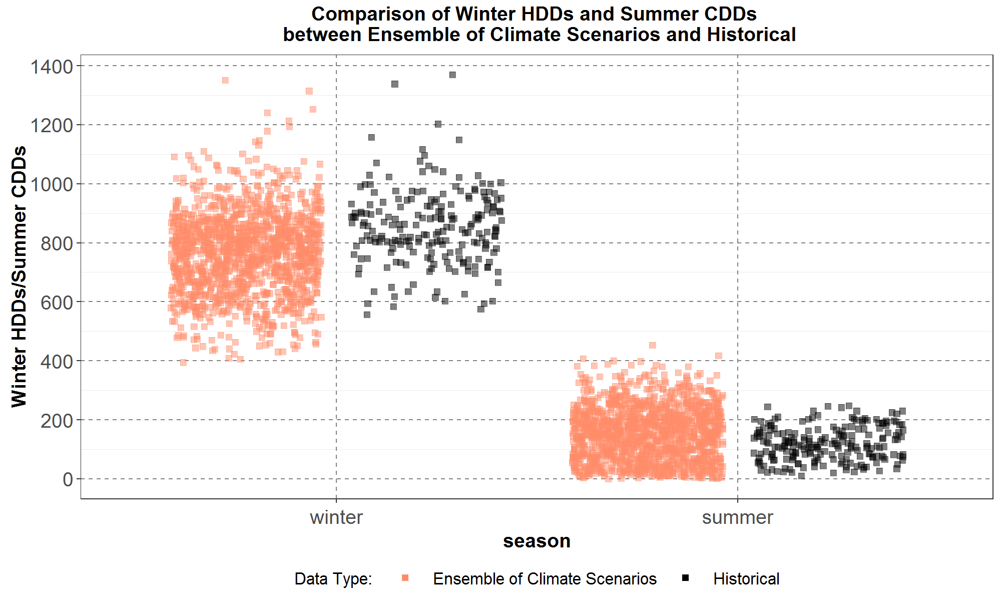
Before starting the scenario selection process, it is worthwhile to compare winter HDDs and summer CDDs between the ensemble of the 15 unique climate scenarios and the historical 70 temperature-years (1948 – 2017). The data are presented in Figure 9, where the ensemble is plotted in orange while the historical is plotted in black, with winter HDDs on the left and summer CDDs on the right. The magnitudes of the HDDs and CDDs are along the y-axis. For each season, the ensemble degree-days contain (3 months) x (30 future years) x (15 scenarios) = 1,350 data points, whereas the historical degree-days have (3 months) x (70 historical temperature-years) = 210 data points.
The plots in in Figure 9 suggest that, compared to the corresponding seasonal historical HDDs and CDDs, the ensemble, on average, has lower HDDs for winter and higher CDDs for summer.
Figure 9: Comparisons of winter HDDs (on the left) and summer CDDs (on the right), between the ensemble of 15 unique climate scenarios for temperature (in orange) and historical (in black). The magnitudes of the HDDs and CDDs are along the y-axis
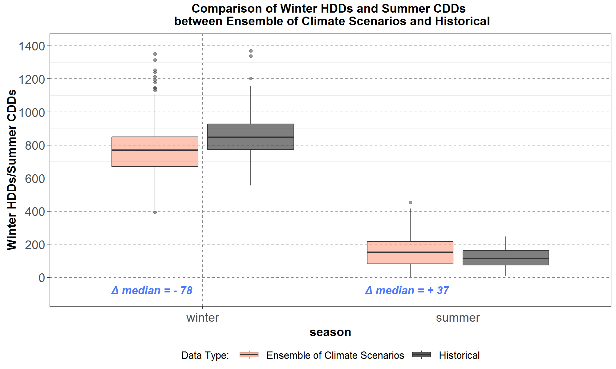
Next, Figure 10 presents the same data as in Figure 9 but in terms of boxplots for quantitative comparisons. For example, the plots show that the ensemble median is 78 degree-days lower than historical median for winter, and in contrast, 37 degree-days higher than historical median for summer. Thus, under the effects of potential future climates, on average, the northwest regional load should be lower for winter and higher for summer.
Figure 10: Comparisons of winter HDDs (on the left) and summer CDDs (on the right), between the ensemble of 15 unique climate scenarios for temperature (in orange) and historical (in black).
The magnitudes of the HDDs and CDDs are along the y-axis. Compared to historical median HDDs and CDDs, the ensemble median HDD is 78 degree-days lower for winter and 35 degree-days higher for summer
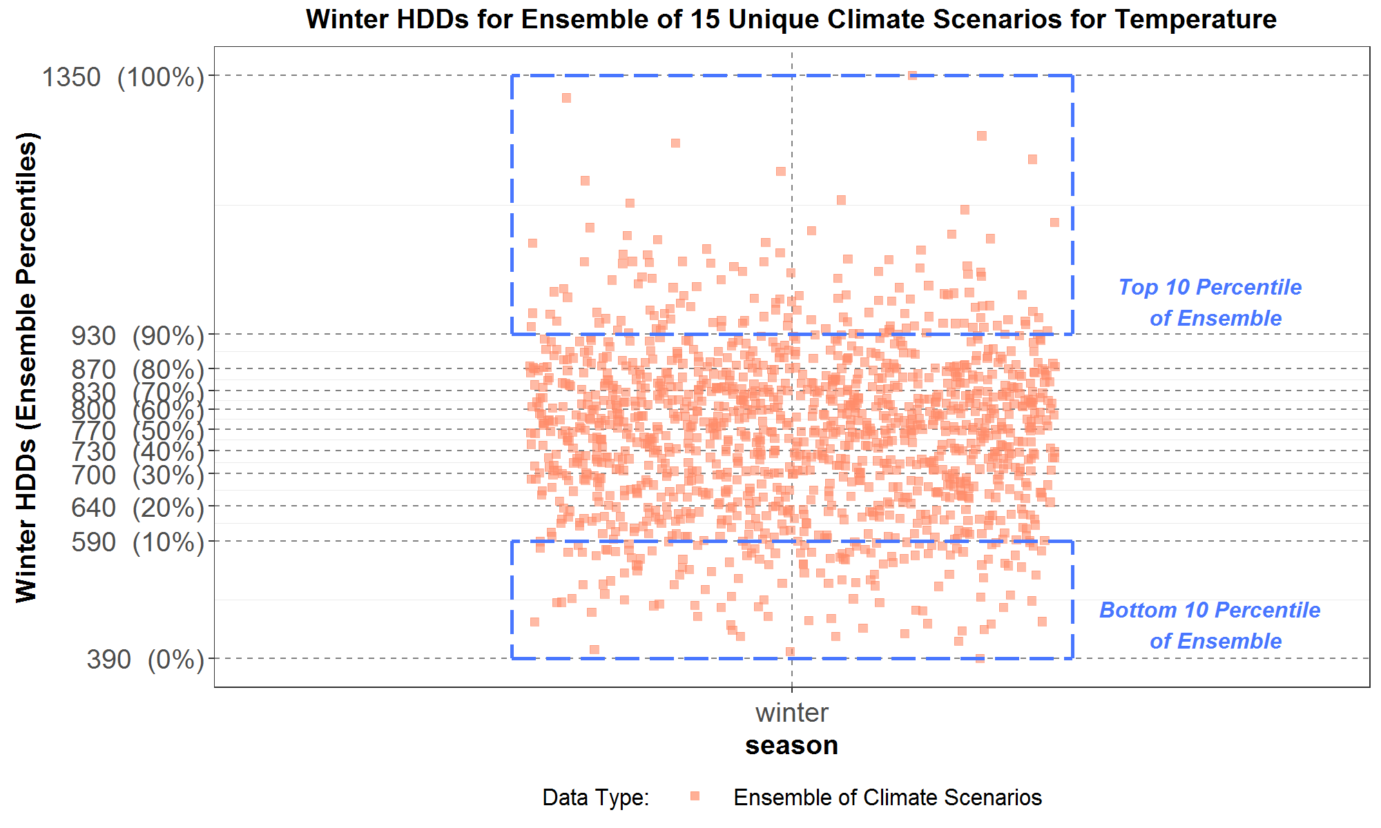
Next in Figure 11, the ensemble winter HDDs in Figure 9 is magnified and the same algorithm described in Figure 4 is applied to select scenarios that represent high and low ensemble winter HDDs. The ensemble winter HDDs has been divided into 10 equal-population slices by the y-axis grid lines with the ensemble deciles printed in parentheses along the y-axis. For example, the bottom-10 percentiles are between 394 HDDs and 587 HDDs and delineated by the lower blue dashed box, while the top-10 percentiles are between 926 HDDs and 1,351 HDDs and delineated by the upper blue dashed box. The algorithm then selects the scenario with the highest population in the bottom-10 percentiles to represent low ensemble winter HDDs. Similarly, the algorithm selects the scenario with the highest population in the top-10 percentiles to represent high ensemble winter HDDs.
Figure 11: The ensemble winter HDDs divided into 10 equal-population slices, or deciles.
The deciles are divided by the y-axis grid lines and printed in parentheses along the y-axis. The bottom-10 and top-10 ensemble percentiles are delineated respectively by the lower and upper blue dashed boxes.
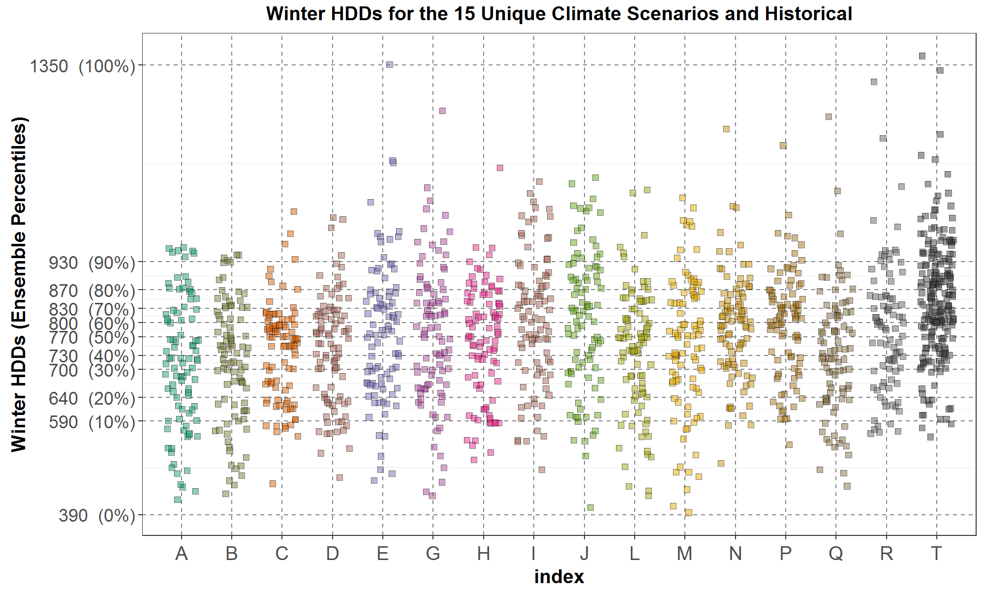
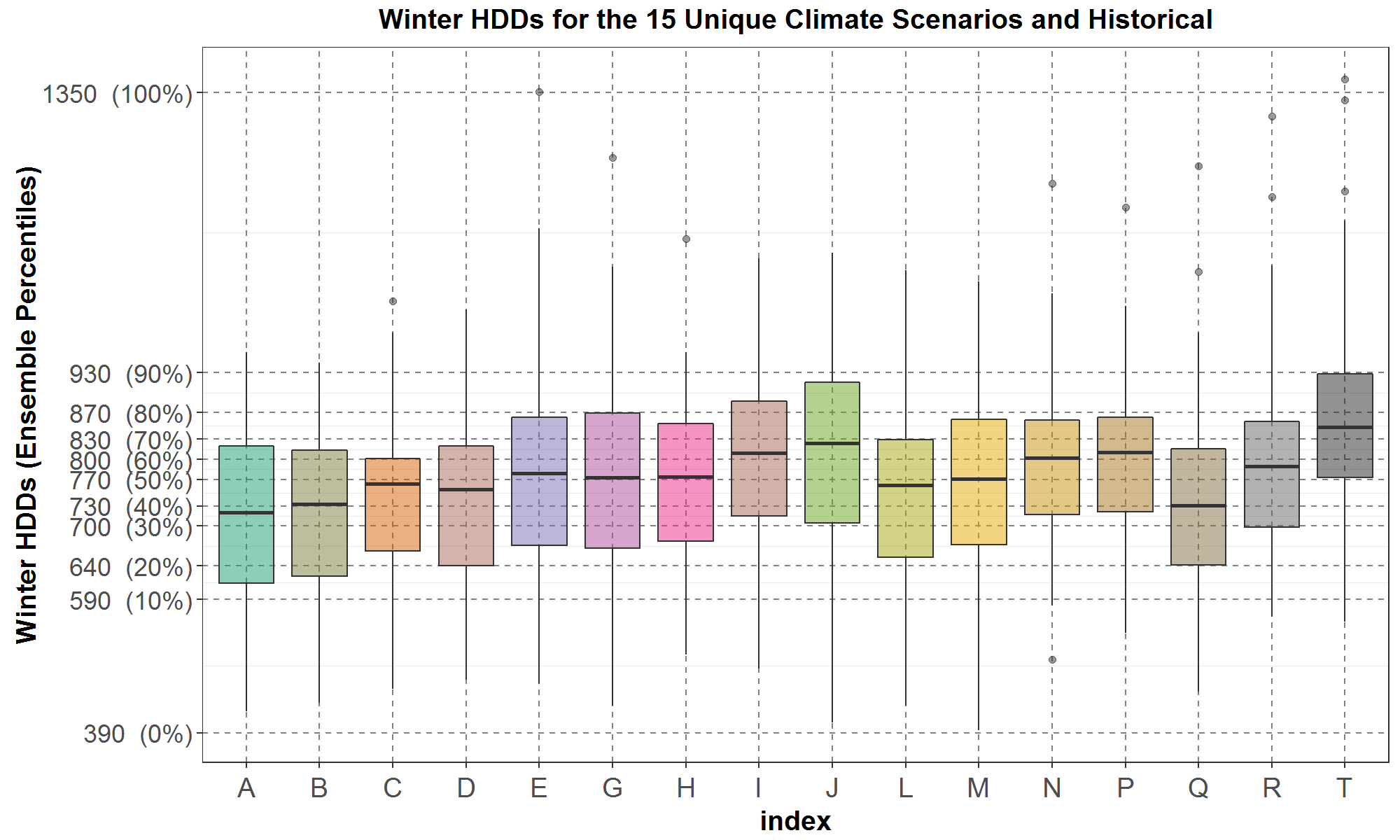
The selection algorithm is demonstrated by breaking up the ensemble winter HDDs in Figure 11 into its components of 15 unique scenarios for temperatures and plotted in Figure 12. The 15 scenarios are listed by scenario indices along the x-axis, from A to R, according to Table 3 in Summary of the RMJOC Climate Scenarios. However, scenarios F, K, O and S are not plotted since their temperature data are duplicates of those in scenarios G, J, N and R, respectively. For comparison, the historical winter HDDs are also plotted as scenario T. The plots suggest that most of the 15 scenarios on average have lower HDDs than historical. Once again, the ensemble deciles are in parentheses along the y-axis. Hence, the algorithm selects the scenario with the most data points between the 0% and the 10% y-axis grid lines, and the scenario with the most data points between the 90% and the 100% grid lines.
Figure 12: Winter HDDs for the 15 unique climate scenarios for temperatures with indices from A to R according to Table 3 in Summary of the RMJOC Climate Scenarios (the duplicate scenarios F, K, O and S are not plotted).
The historical winter HDDs are also plotted and have index T. The y-axis grid lines are deciles of the ensemble winter HDDs
Results of the population counts for each scenario (except for the excluded I and J) in the bottom-10 and top-10 ensemble percentiles in Figure 12 are listed in Table 5 below.
Table 5: Population of the 13 climate scenarios within the bottom-10 and top-10 ensemble percentiles for winter HDDs.
| Scenario Index | Population in the Bottom-10 Ensemble Percentiles | Population in the Top-10 Ensemble Percentiles | Scenario Index | Population in the Bottom-10 Ensemble Percentiles | Population in the Top-10 Ensemble Percentiles |
| A | 18 | 7 | M | 11 | 9 |
| B | 16 | 6 | N | 3 | 7 |
| C | 8 | 4 | P | 1 | 8 |
| D | 9 | 4 | Q | 14 | 3 |
| E | 6 | 12 | R | 6 | 14 |
| G | 8 | 14 | |||
| H | 9 | 5 | |||
| L | 14 | 6 |
In Table 5, scenario A has the highest population in the bottom-10 ensemble percentiles, at 18, and is thus selected to represent low ensemble winter HDDs.
On the other hand, scenarios G and R have the highest population in the top-10 ensemble percentiles, at 14. Furthermore, because in the previous section G had already been selected to represent low winter and high summer generation, G then is also selected to represent high winter HDDs to reduce the total number of scenarios included for power plan analyses.
For more quantitative comparisons of the distributions, the same data in Figure 12 are presented in boxplots in Figure 13. It shows that the historical HDD (scenario T) central percentiles, represented by the dark gray box, are higher than the corresponding percentiles for all 15 climate scenarios. Thus, as expected, all the climate scenarios have warmer winters than historical, on average.
Figure 13: Winter HDDs for the 15 unique climate scenarios for temperatures with indices from A to R according to Table 3 in Summary of the RMJOC Climate Scenarios (the duplicate scenarios F, K, O and S are not plotted).
The historical winter HDDs are also plotted and have index T. The y-axis grid lines are deciles of the ensemble winter HDDs
After selecting A and G to represent low and high ensemble winter HDDs, the algorithm is next applied to the ensemble summer CDDs to select its representative low and high scenarios. Summer CDDs for the 15 unique scenarios for temperature are plotted in Figure 14. And similar to the two previous figures, each of the 15 scenarios is listed by its index along the x-axis according to Table 3 in Summary of the RMJOC Climate Scenarios, with the historical summer CDDs plotted as scenario T. The ensemble summer CDD deciles are in parentheses along the y-axis. Among the remaining scenarios after excluding I and J, the algorithm selects the scenario with the most data points between the 0% and the 10% grid lines, and the scenario with the most data points between the 90% and the 100% grid lines.
Figure 14: Summer CDDs for the 15 unique climate scenarios for temperature.
The indices along the x-axis are from Table 3 in Summary of the RMJOC Climate Scenarios (the duplicate scenarios F, K, O and S are not plotted). The historical summer CDDs are also plotted and have index T. The y-axis grid lines are deciles of the ensemble summer CDDs
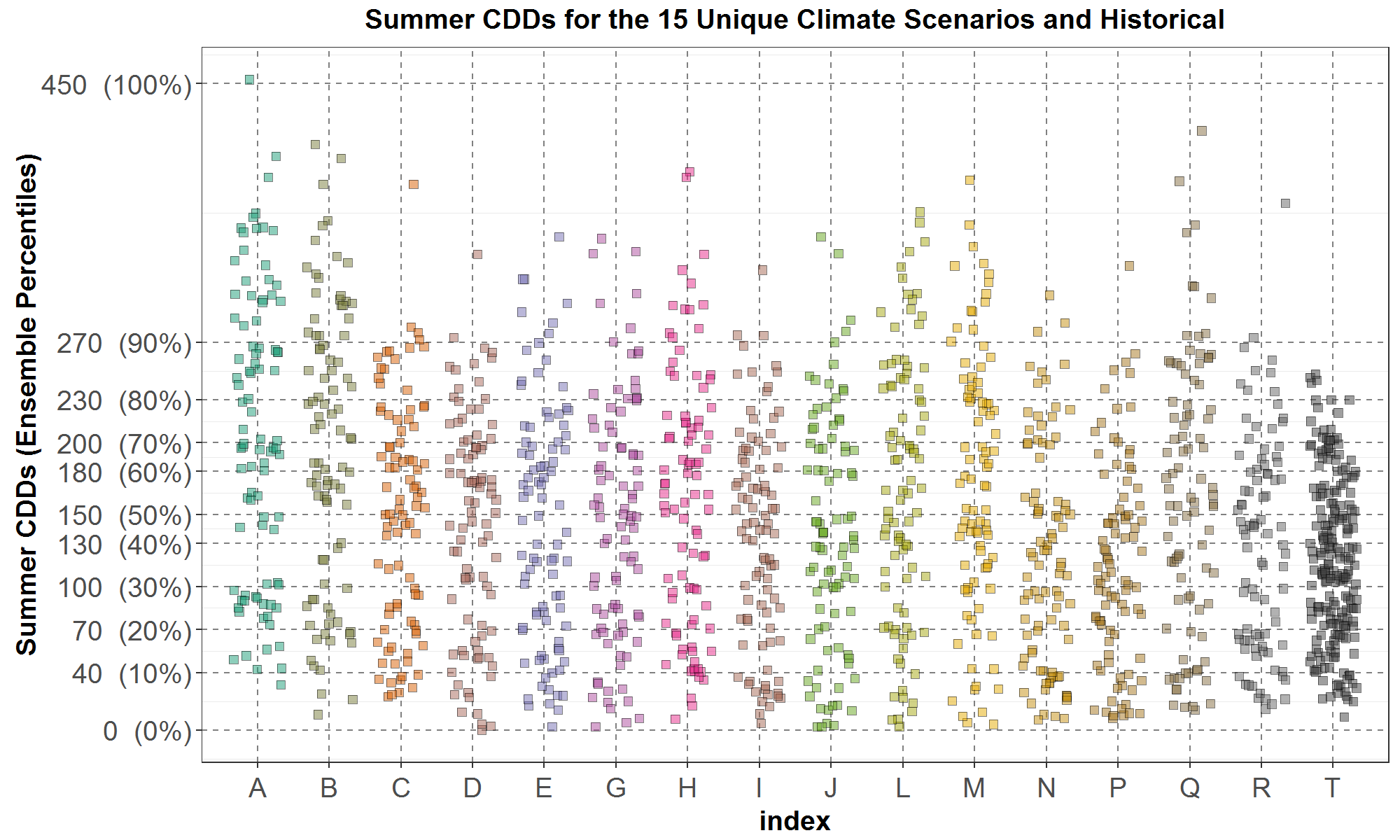
Table 6 below lists the population count for each scenario (except for I and J) in the bottom-10 and top-10 ensemble percentiles in Figure 14.
Table 6: Population of the 13 climate scenarios within the bottom-10 and top-10 ensemble percentiles for summer CDDs.
| Scenario Index | Population in the Bottom-10 Ensemble Percentiles | Population in the Top-10 Ensemble Percentiles | Scenario Index | Population in the Bottom-10 Ensemble Percentiles | Population in the Top-10 Ensemble Percentiles |
| A | 1 | 25 | M | 8 | 14 |
| B | 3 | 25 | N | 14 | 3 |
| C | 7 | 4 | P | 14 | 1 |
| D | 9 | 2 | Q | 10 | 10 |
| E | 9 | 8 | R | 10 | 2 |
| G | 11 | 7 | |||
| H | 4 | 12 | |||
| L | 8 | 14 |
From Table 6, scenarios N and P have the highest population in the bottom-10 ensemble percentiles, at 14, with G having the next highest population at 11. Since scenario G has already been selected to represent not only low ensemble winter and high ensemble summer hydro generation, but also high ensemble winter HDDs, it is also selected to represent low ensemble summer CDDs (as an approximation). Thus, scenario G occupies four of the eight slots in Table 1, helping to reduce the total number of scenarios needed for the Power Plan. It will be analyzed in a subsequent section if selecting scenario G, instead of N or P, would introduce a bias in the finalized set of selected scenarios.
Also from Table 6, scenarios A and B have the highest population in the top-10 ensemble percentiles, at 25. But since A has already been selected to represent low ensemble winter HDDs (see Table 5), it is also selected to represent high ensemble summer CDDs.
Therefore, the algorithm selected G to represent both high ensemble winter HDDs and low ensemble summer CDDs (as an approximation), and conversely selected A to represent both low ensemble winter HDDs and high ensemble summer CDDs. A and G occupy the four slots for winter HDDs and summer CDDs as shown in Table 1.
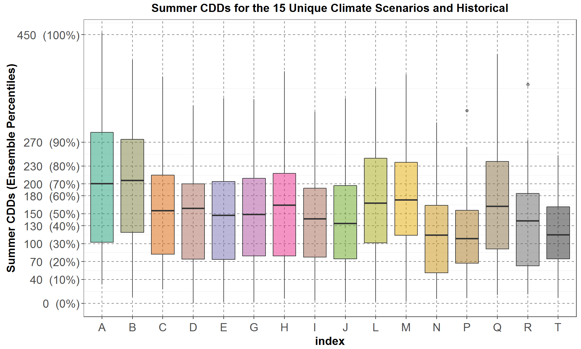
Finally, Figure 15 presents the same summer CDD data as Figure 14 in boxplots. It shows that all scenarios have higher maxima than historical, and except for N and P, also have higher 75th percentiles and medians than historical. Thus, most of the climate scenarios have significantly warmer summers than historical, on average.
Figure 15: Summer CDDs for the 15 unique climate scenarios for temperature. The indices along the x-axis are from Table 3 in Summary of the RMJOC Climate Scenarios (the duplicate scenarios F, K, O and S are not plotted).
The historical summer CDDs are also plotted and have index T. The y-axis grid lines are deciles of the ensemble summer CDDs
Properties of the Selected Scenarios
In the previous section, scenarios were selected based on having (approximately) the most population in the top-10 and bottom-10 ensemble percentiles for the four variables: winter and summer hydro generation, winter HDDs and summer CDDs. The selected scenarios then represent the high and low of the four ensemble distributions. However, some scenarios were excluded and some were replaced in the selection process, and thus, in this section the selected scenarios are analyzed to determine if they, as a group, are good representations of the ensemble of the 19 RMJOC scenarios. In addition, for each of the four variables of interests, the distributions for the selected scenarios are also individually compared with the climate ensemble and historical distributions.
Winter and Summer Hydro-Generation of Scenarios C and G and the Climate Ensemble
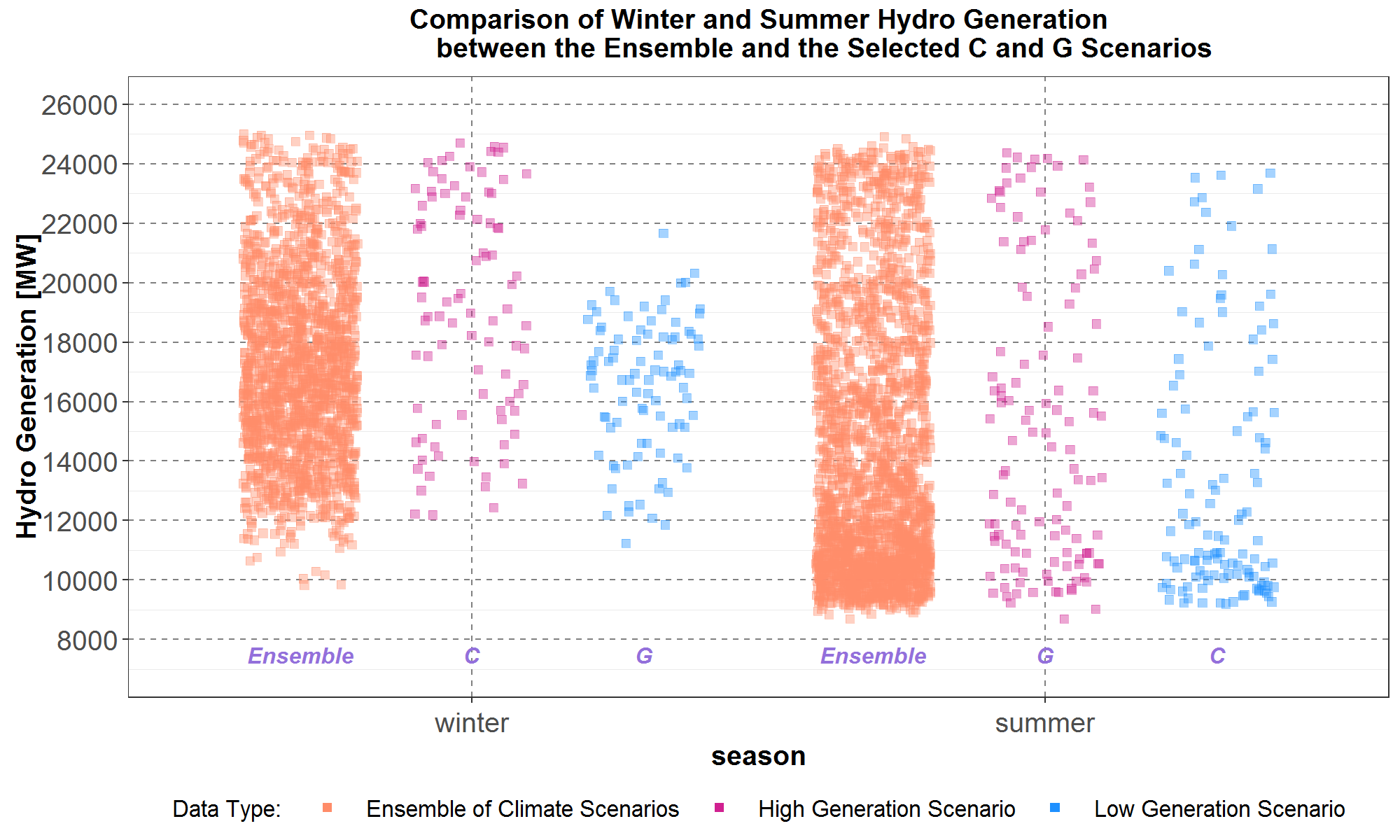
To represent high and low ensemble winter and summer hydro generations, the algorithm selected scenarios C and G (as an approximation for low winter hydro generation after scenarios I, J and K were excluded). Their distributions are compared to the ensemble distributions, in terms of jitter plots in Figure 16, and in terms of boxplots in Figure 17.
In Figure 16, only the winter generations for scenario G, with very few data points above 20,000 MW, could be considered outliers of the ensemble winter generations. The remaining scenarios have similar seasonal ranges as the corresponding ensemble distribution and thus would not be considered as outliers.
Figure 16: Comparisons of winter (left side) and summer (right side) generations between the selected scenarios (C and G) and the ensemble.
The ensemble generations are in orange, the representative high-generation scenarios (both winter and summer) are in pink and the representative low-generation scenarios are in blue
In Figure 17, the blue boxplot on the left, which represents the distribution of winter generations for scenario G, has a slightly smaller range than the ensemble distribution, in the orange boxplot. However, as both plots have nearly the same median and both boxes have similar ranges, then G should not be considered an outlier of the winter ensemble. On the other hand, the pink boxplot on the left, representing C, has a significantly higher box than that for the ensemble, but its distribution is probably not too extreme in comparison to the ensemble distribution to be considered as an outlier. For the two summer scenario distributions on the right side, although they have slightly different ranges in boxes and whiskers than those for the ensemble, there is nevertheless enough overlap with the ensemble that should preclude them from being considered as outliers.
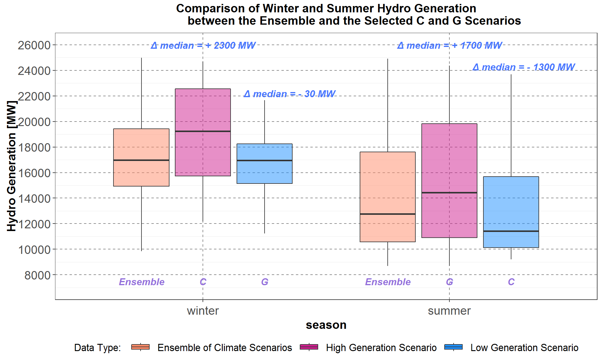
For numerical comparisons of the medians, Figure 17 shows that for winter, relative to the ensemble, the high-generation scenario C is 2,300 MW higher while the low-generation scenario G is only 30 MW lower. And for summer the high-generation scenario G is 1,700 MW higher while the low-generation scenario C is 1,300 MW lower.
Figure 17: Comparisons of winter (left side) and summer (right side) generations between the selected scenarios (C and G) and the ensemble. The ensemble generations are in orange, the representative high-generation scenarios (both winter and summer) are in pink and the representative low-generation scenarios are in blue. Above the top whisker of each scenario is the difference between its median and the ensemble median
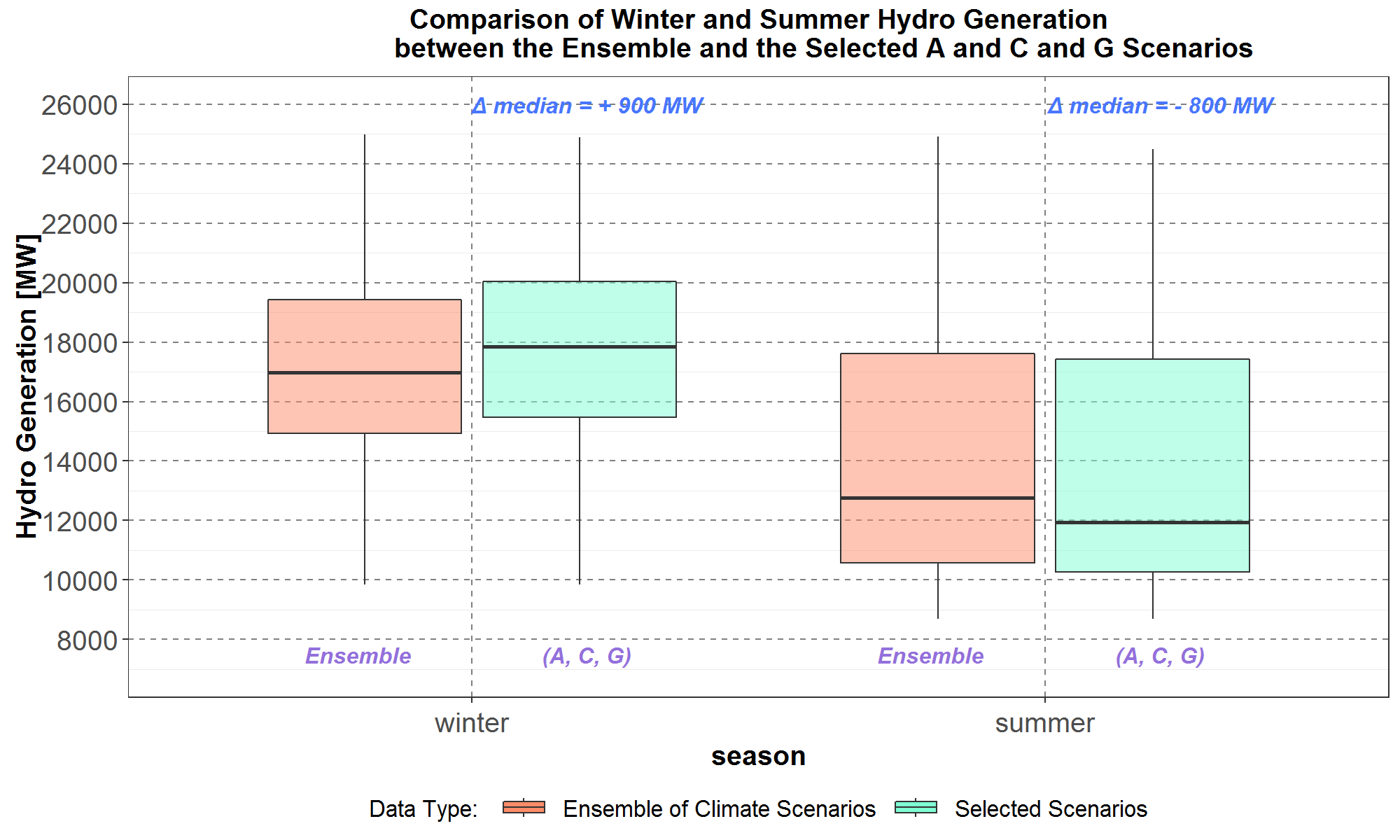
Even though scenarios C and G were selected to represent high and low ensemble winter and summer hydro generations, it is important to determine that the selected scenarios, as a group, could reasonably resemble the ensemble distribution and do not contain significant bias. Thus, Figure 18 is a very similar plot to Figure 17 where the green boxplots represent hydro generation distributions of both scenarios C and G. The comparisons show that, in terms of boxplot statistics, hydro generations from scenarios C and G, as a group, are somewhat close to the ensemble distribution (in the orange boxplot) for winter, and very close to the ensemble distribution for summer. More specifically, for winter, the differences between the maxima (tops of the upper whiskers), the 75th, 50th (the median) and 25th percentiles are less than or equal to 700 MW. However, the difference between the minima (bottoms of the lower whiskers) is larger, at 1400 MW. On the other hand, for summer, the differences between the minima, 25th, 50th and 75th percentiles are around 200 MW or smaller, while the difference between the maxima is slighter larger, at 500 MW.
Figure 18: Comparisons of winter (left side) and summer (right side) generations between the selected scenarios (C and G) as a group and the ensemble.
The ensemble generations are in orange and the selected scenario generations are in green. Above the top whisker of the selected scenarios is the difference between its median and the ensemble median
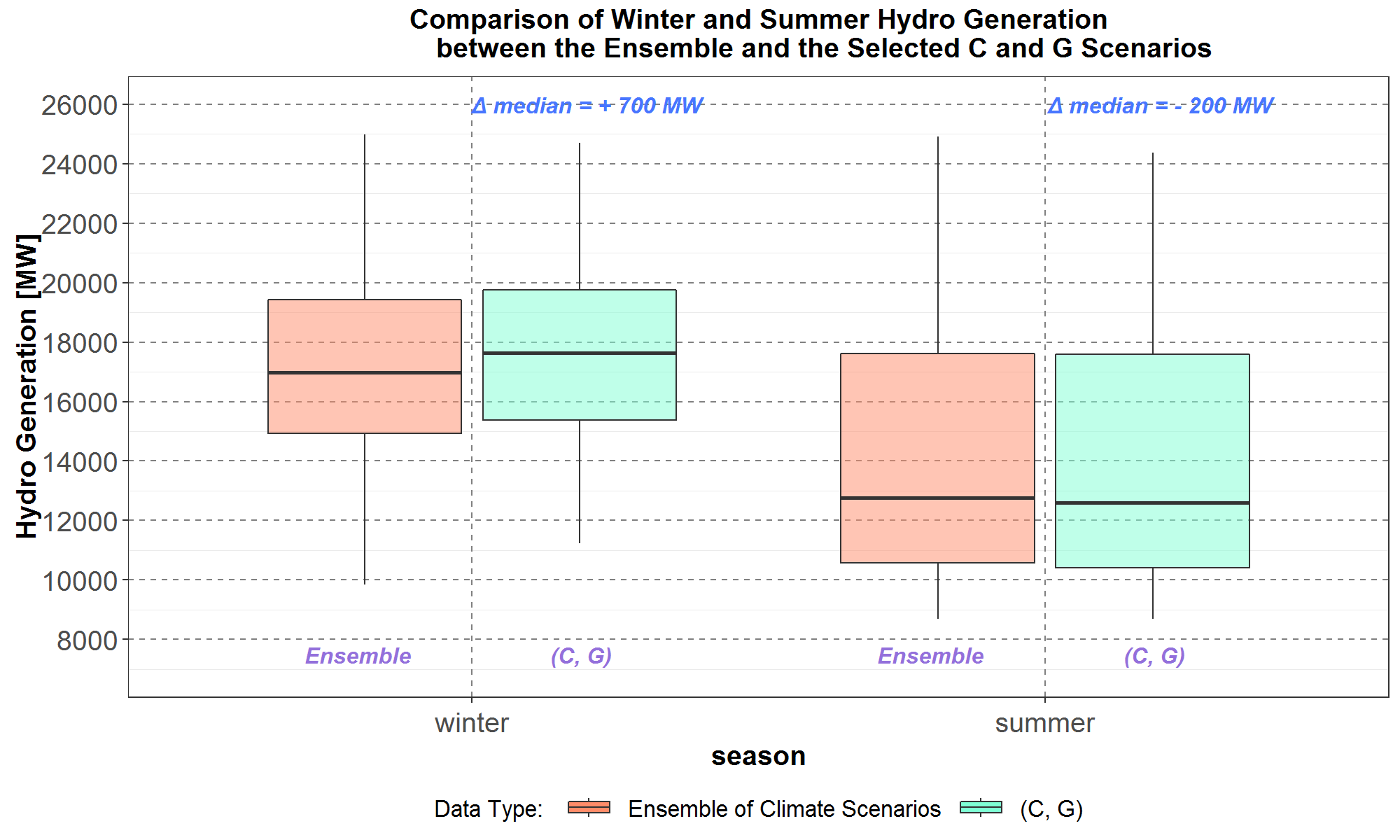
Therefore, the selected scenarios C and G as a group can reasonably represent the ensemble winter hydro generation and can very well represent the ensemble summer hydro generation.
Winter HDDs and Summer CDDs of Scenarios A and G and the Climate Ensemble
Next is an analysis of properties of the climate scenarios selected to represent high and low ensemble winter HDDs and summer CDDs.
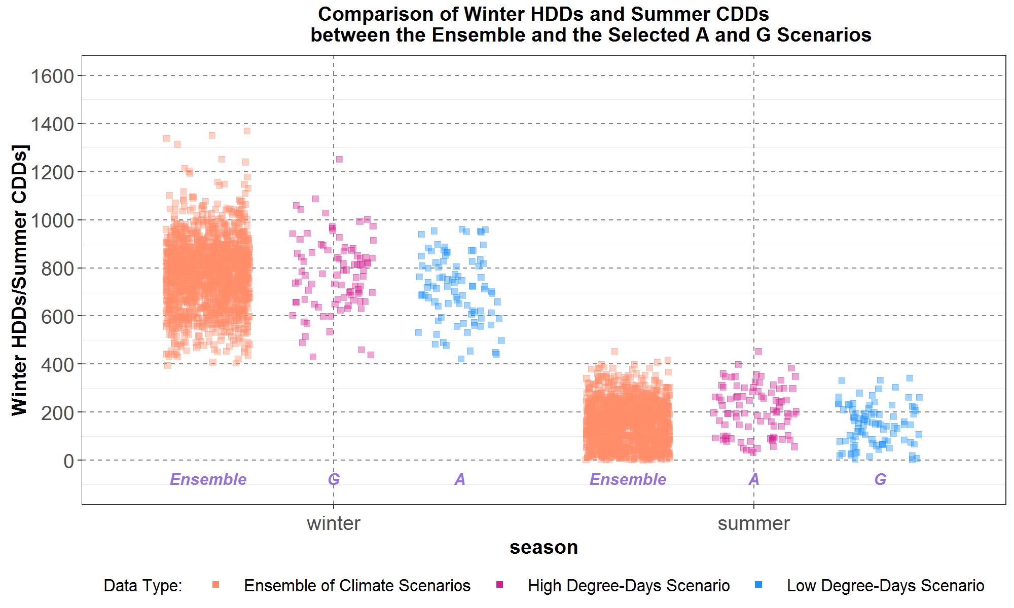
Since the algorithm selected scenarios A and G (as an approximation to represent low ensemble summer CDDs, replacing scenarios N and P), then their distributions are compared with the ensemble distributions in terms of jitter plots in Figure 19, and boxplots in Figure 20.
In Figure 19, scenario A in winter has a smaller range than the ensemble due to it having no data greater than 1,000 HDDs. However, between 400 and 1,000 HDDs, there is enough overlap with the ensemble winter HDDs that A should not be considered an outlier of the ensemble. Otherwise, the remaining scenarios have similar seasonal degree-day ranges as the corresponding ensemble distribution and thus do not look like outliers.
Figure 19: Comparisons of winter HDDs (left side) and summer CDDs (right side) between the selected scenarios (A and G) and the ensemble.
The ensembles are in orange, the representative high degree-days scenarios (both winter and summer) are in pink and the representative low degree-days scenarios are in blue
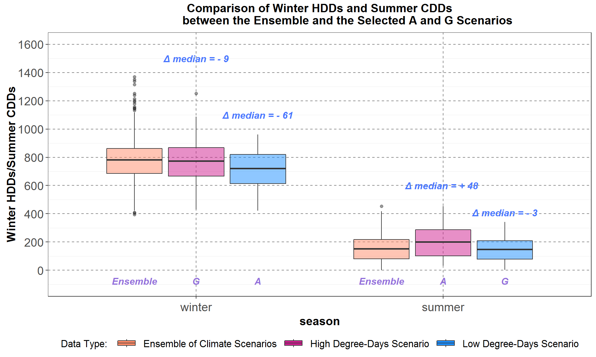
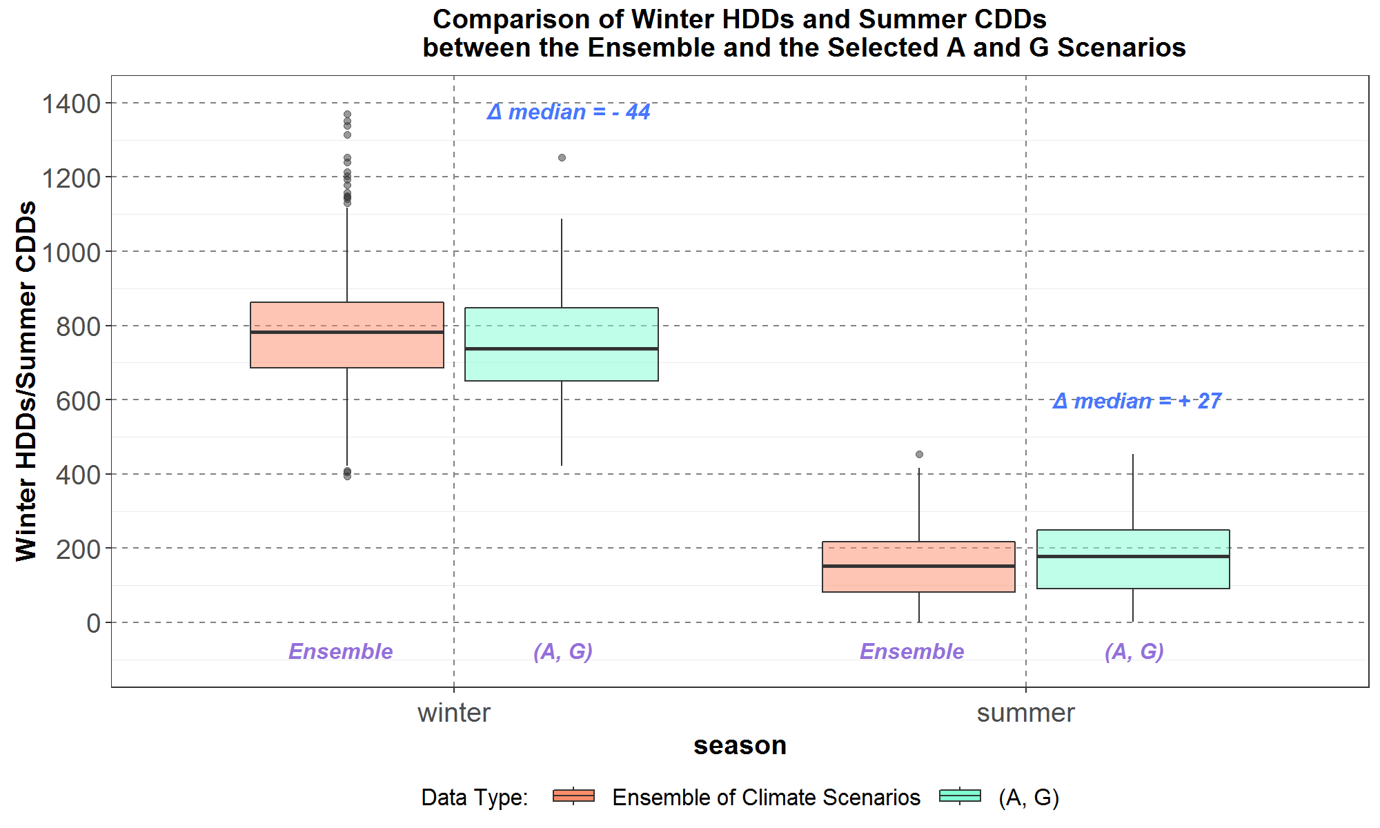
Next, the boxplots in Figure 20 show very substantial overlaps among all the distributions for each season and thus also support scenarios A, G not being outliers of the ensembles. Furthermore, numerical comparisons of the medians show that for winter, relative to the ensemble, the high-HDD scenario G is 9 lower (the excluded scenarios I and J have higher median HDDs than the ensemble) while the low-HDD scenario A is 61 lower. And relative to the ensemble summer median, the high-CDD scenario A is 48 higher while the low-CDD scenario G is 3 lower. Visual comparisons of other boxplot statistics also suggest that scenarios A and G are not outliers of the ensemble distributions for winter HDDs and summer CDDs.
Figure 20: Comparisons of winter HDDs (left side) and summer CDDs (right side) between the selected scenarios (A and G) and the ensemble.
The ensembles are in orange, the representative high degree-days scenarios (both winter and summer) are in pink and the representative low degree-days scenarios are in blue. Above the top whisker of each scenario is the difference between its median and the ensemble median
Finally, the winter HDD and summer CDD distributions of scenarios A and G, as a group, are analyzed to determine if they could reasonably represent the ensemble degree-day distributions of the 15 RMJOC scenarios and do not contain significant bias.
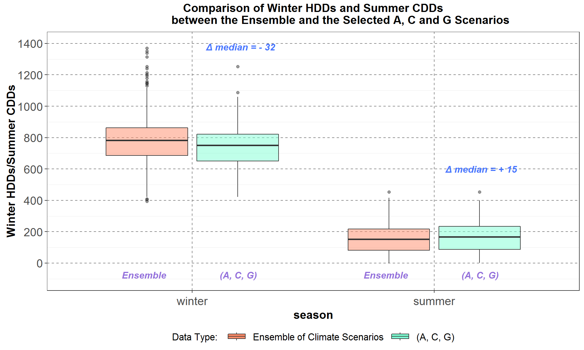
Figure 21 shows that, in terms of boxplot statistics, distributions of winter HDDs and summer CDDs from scenarios A and G (as a group in the green boxplots) are close to the ensemble distributions (in the orange boxplots) for both winter and summer. More specifically, for winter, the differences between the minima (lowest outlier for the ensemble and bottom of the lower whisker for A and G), 25th, 50th and 75th percentiles are less than or equal to 44 HDDs. However, the difference between the maxima (highest outlier for the ensemble and top of the upper whisker for A and G) is larger, at 117 HDDs. On the other hand, for summer, the differences between all the boxplot statistics, the minima, the 25th, 50th and 75th percentiles and the maxima are 33 CDDs or smaller.
Figure 21: Comparisons of winter (left side) and summer (right side) degree-days between the selected scenarios (A and G) as a group and the ensemble. The ensemble degree-days are in orange and the selected scenario degree-days are in green. Above the top whisker of the selected scenarios is the difference between its median and the ensemble median
Thus, visual and numerical comparisons of the boxplots in Figure 21 support that the selected scenarios A and G as a group can represent the ensemble winter HDDs and summer CDDs.
Winter and Summer Hydro-Generation and Degree-Days of Scenarios A, C and G and the Climate Ensemble
In summary, Table 7 below lists the high and low of the ensemble distributions for winter and summer hydro generations, and winter HDDs and summer CDDs that the selected scenarios A, C and G represent. All three scenarios by design occupy more than one slot across the four variables to reduce the total number of scenarios for analysis in the Power Plan.
Table 7: Summary of the selected scenarios A, C and G
| Scenario | Winter Hydro Generation | Summer Hydro Generation | Winter HDDs | Summer CDDs |
| A | low | high | ||
| C | high | low | ||
| G | low | high | high | low |
However, according to Tables 5 and 6, scenario A has the second highest population in the top-10 percentiles of ensemble winter hydro generation and is tied with scenario C for having the highest population in the bottom-10 percentiles of ensemble summer hydro generation. Thus, for winter and summer hydro generations, scenario A resembles scenario C. Thus, as a group, the selected scenarios A, C and G could be approximated as consisting of two C’s and one G. The consequence is that, as presented in Figure 22, the green boxplots for the A, C and G group are displaced further away from the orange ensemble boxplots compared to those in Figure 18. More specifically, relative to the ensemble boxplots, the A, C, G grouped boxplots are displaced higher for winter and lower for summer.
Figure 22: Comparisons of winter (left side) and summer (right side) generations between the selected scenarios (A, C and G) as a group and the ensemble. The ensemble generations are in orange and the selected scenario generations are in green. Above the top whisker of the selected scenarios is the difference between its median and the ensemble median
Next, Tables 7 and 8 show that the HDD and CDD values for scenario C are not close to those of the scenarios A and G which represent the highs and lows of the ensemble degree-day distributions. Thus, scenario C could be considered being somewhere in the “middle” of the ensemble distribution. And the result, as presented in Figure 23, is that adding scenario C to A and G pulls the A, C and G group distributions in the green boxplots to be closer to the ensemble distributions compared to those in Figure 21.
Figure 23: Comparisons of winter (left side) and summer (right side) degree-days between the selected scenarios (A, C and G) as a group and the ensemble.
The ensemble degree-days are in orange and the selected scenario degree-days are in green. Above the top whisker of the selected scenarios is the difference between its median and the ensemble median
Finally, the GCM, downscaling method and hydrological models used for scenarios A, C and G are listed in Table 8, which is a smaller version of Table 3 in Summary of the RMJOC Climate Scenarios.
Table 8: The GCM, downscaling method and hydrological model for scenarios A, C and G
| Scenario Index | Scenario |
| A | CanESM2_RCP85_BCSD_VIC_P1 |
| C | CCSM4_RCP85_BCSD_VIC_P1 |
| G | CNRM-CM5_RCP85_MACA_VIC_P3 |
Winter and Summer Hydro-Generation and Degree-Days of Scenarios A, C and G and the Historical
As discussed in a previous section, for the Power Plan, relevant data from the three scenarios are incorporated into various Council models whose outputs are analyzed. Among that work is assessing the northwest power system adequacy under the influence of a set of possible of future climates represented by the scenarios. However, it might be useful to also analyze qualitative trends in system adequacy from the four variables: winter and summer hydro generation, winter HDDs and summer CDDs. Therefore, for the three selected scenarios, their distributions are compared with those for the historical.
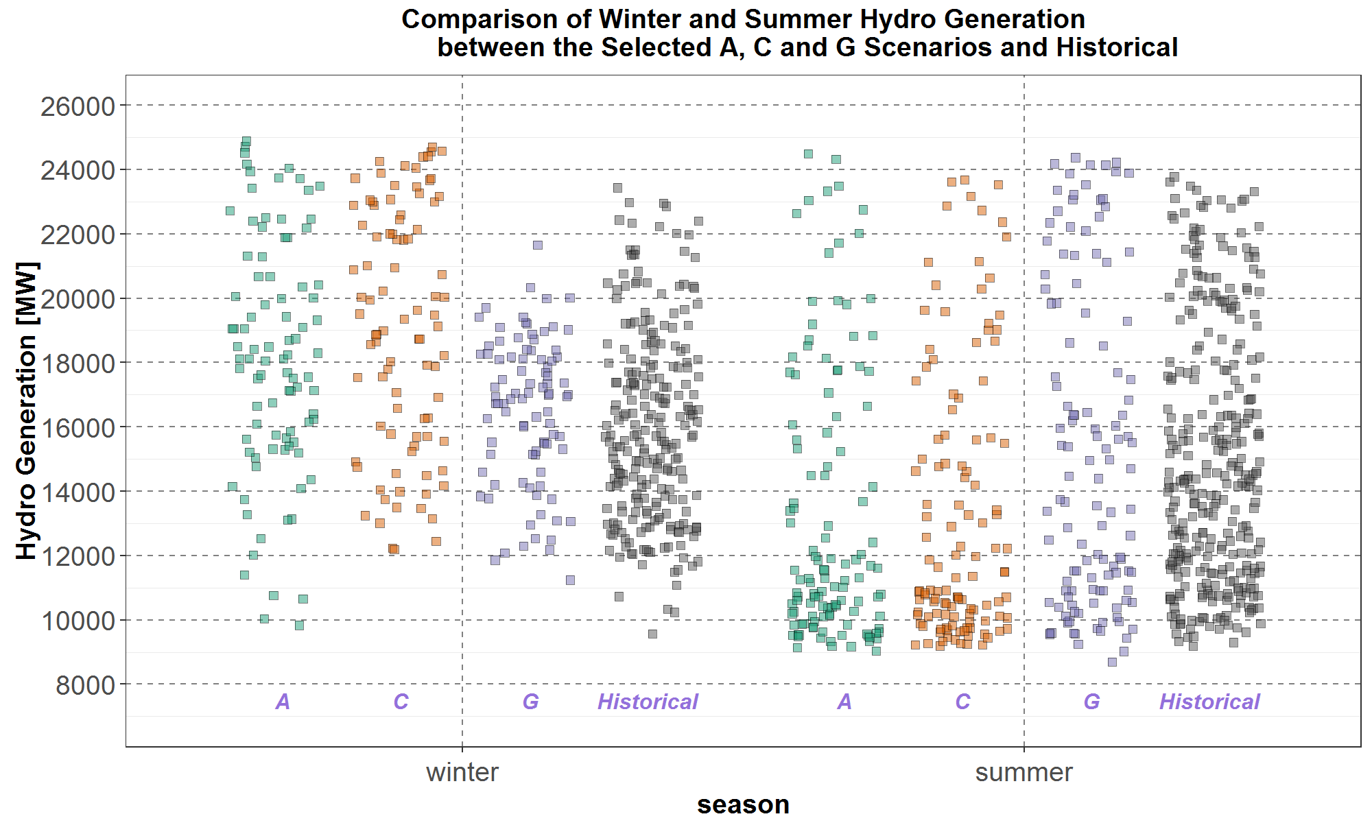
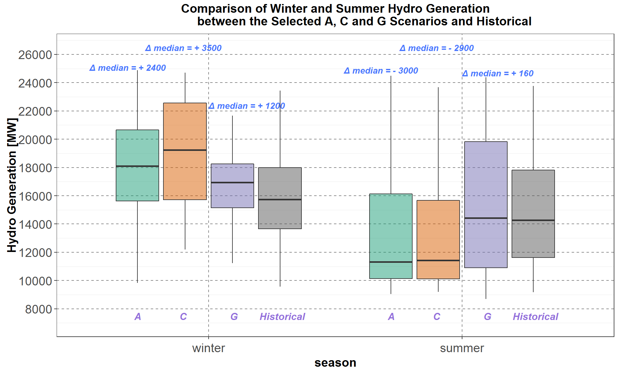
In Figure 24 below, the distributions of winter and summer hydro generations for the three scenarios are compared with the corresponding historical distribution. It shows that, on average, scenarios A and C have higher winter and lower summer generation than historical, whereas for G, the comparison is not as clear.
Figure 24: Comparisons of winter hydro generation (left side) and summer hydro generation (right side) between the selected scenarios A, C and G and the historical. The historical generations are in black, A in green, C in brown and G in blue
In Figure 25, the same distributions in Figure 24 are plotted as boxplots to enable quantitative comparisons. In terms of medians (the black line inside each box), all three scenarios are thousands of megawatts higher than historical for winter. Conversely, for summer, scenarios A and C are thousands of megawatts lower than historical, while G is somewhat comparable to historical.
Figure 25: Comparisons of winter hydro generation (left side) and summer hydro generation (right side) between the selected scenarios A, C and G and the historical.
The historical generations are in black, A in green, C in brown and G in blue. Above the top whisker of each scenario is the difference between its median and the historical median
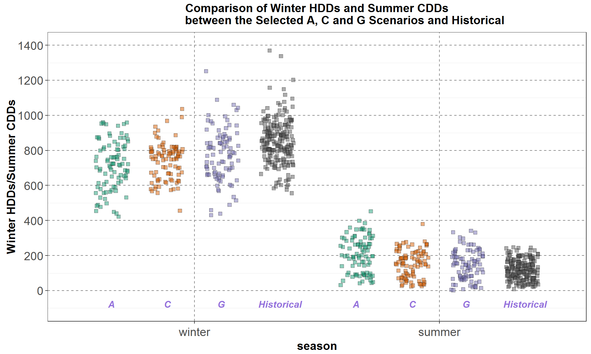
Next, in Figure 26 are comparisons of winter HDDs and summer CDDs between the selected scenarios and historical. All three scenarios, on average, seem to have lower winter HDDs and higher summer CDDs.
Figure 26: Comparisons of winter HDDs (left side) and summer CDDs (right side) between the selected scenarios A, C, and G and the historical. The historical degree-days are in black, A in green, C in brown and G in blue
Finally, in Figure 27, the same distributions in Figure 26 are plotted as boxplots. From comparing the medians (the black line inside the box), scenario A has the highest warming, with 127 fewer winter HDDs and 86 more summer CDDs than historical. The other two scenarios, C and G, have comparable warming, with about 80 fewer winter HDDs and about 40 more summer CDDs than historical.
Figure 27: Comparisons of winter HDDs (left side) and summer CDDs (right side) between the selected scenarios A, C, and G and the historical.
The historical degree-days are in black, A in green, C in brown and G in blue. Above the top whisker of each scenario is the difference between its median and the historical median
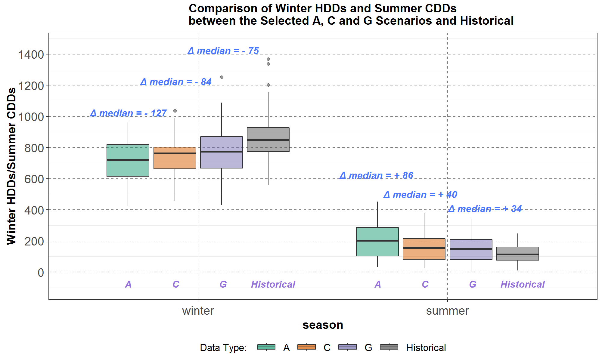
Figures 24 to 27 suggest that power system adequacy under the influence of the climate scenarios should be easier to achieve for winter due to having, on average, higher hydro generation and lower load (due to lower winter HDDs) than historical. On the other hand, adequacy for summer should be worse because of lower hydro generation (except for scenario G) and higher loads (from higher summer CDDs) than historical.
More detailed analyzes of streamflows and temperatures for the three climate scenarios are available in trends in climate hydro and trends in climate temperature respectively.
See also this spreadsheet: The 10 Lowest winter and 10 Lower Summer Classic GENESYS Hydro Generation Among the Selected Climate Scenarios and Historical