


Overview
Since 2017, historical hourly regional temperatures from 1948 onward have been used to produce regional hourly load forecasts for use in resource adequacy studies. For the 2021 Power Plan, the Council instead used forecasted future climate data developed by the River Management Joint Operating Committee (RMJOC). A comprehensive report on the RMJOC climate data is available in the RMJOC report I. However, the RMJOC temperature data only provide daily maximums and minimums, and thus Council staff developed a methodology to transform the RMJOC daily temperatures into hourly temperatures for use in the Council’s load forecast model and energy efficiency building simulation models. The following sections contain analysis of the climate data and a description of the methodology.
The Regional Temperature
The regional temperature is of particular interest since it is an input of the Council’s load forecast model. The regional temperature T is not the temperature at any specific location, but a weighted sum of temperatures at four Northwest cities – Seattle, Washington, Portland, Oregon, Spokane, Washington, and Boise, Idaho - and a constant term and is expressed as follows:
T = a*TSeattle+ b*TPortland+ c*TSpokane+ d*TBoise+ k (1)
where coefficients a , b , c , d and constant k vary by month as indicated in Table 3 below.
Table 3: Monthly coefficients a , b , c , d and constant term k for transforming temperatures for Seattle, Portland, Spokane, and Boise to the regional temperature
| Month | a | b | c | d | k |
| 1 | 0.492 | 0.258 | 0.219 | 0.062 | -2.544 |
| 2 | 0.492 | 0.258 | 0.219 | 0.062 | -2.544 |
| 3 | 0.492 | 0.258 | 0.219 | 0.062 | -2.544 |
| 4 | 0.492 | 0.258 | 0.219 | 0.062 | -2.544 |
| 5 | 0.352 | 0.192 | 0.203 | 0.150 | 6.542 |
| 6 | 0.352 | 0.192 | 0.203 | 0.150 | 6.542 |
| 7 | 0.337 | 0.230 | 0.218 | 0.103 | 7.343 |
| 8 | 0.337 | 0.230 | 0.218 | 0.103 | 7.343 |
| 9 | 0.337 | 0.230 | 0.218 | 0.103 | 7.343 |
| 10 | 0.414 | 0.127 | 0.175 | 0.122 | 9.573 |
| 11 | 0.414 | 0.127 | 0.175 | 0.122 | 9.573 |
| 12 | 0.147 | 0.443 | 0.152 | 0.046 | 6.391 |
According to Table 3, in most months, Seattle’s temperature provides the largest contribution to the overall regional temperature since its coefficients, a, are the largest. Next, the Portland and Spokane temperatures provide comparable contributions since their coefficients, b and c , in general have similar magnitudes and rank second and third respectively, and finally, the Boise temperature provides the smallest contribution since its coefficient, d, is the smallest. The monthly coefficients, a, b , c , and d were derived based on ratios of historical monthly loads among the four Northwest cities.
Transforming Daily Regional Temperatures to Hourly Regional Temperatures
This section references materials from Summary of the RMJOC Climate Scenarios.
Regional daily minimum and maximum temperatures are calculated from the RMJOC climate scenario temperatures for the four cities using Equation (1). As an example, Figure 1 shows the downscaled regional temperatures for the CCSM4 Global Climate Model (GCM) with RCP 8.5 and the BCSD downscaling method for the future year 2035. This downscaled GCM has the same temperatures as climate scenario C in Table 3 of Summary of the RMJOC Climate Scenarios, which is one of the RMJOC climate scenarios selected for the Power Plan.
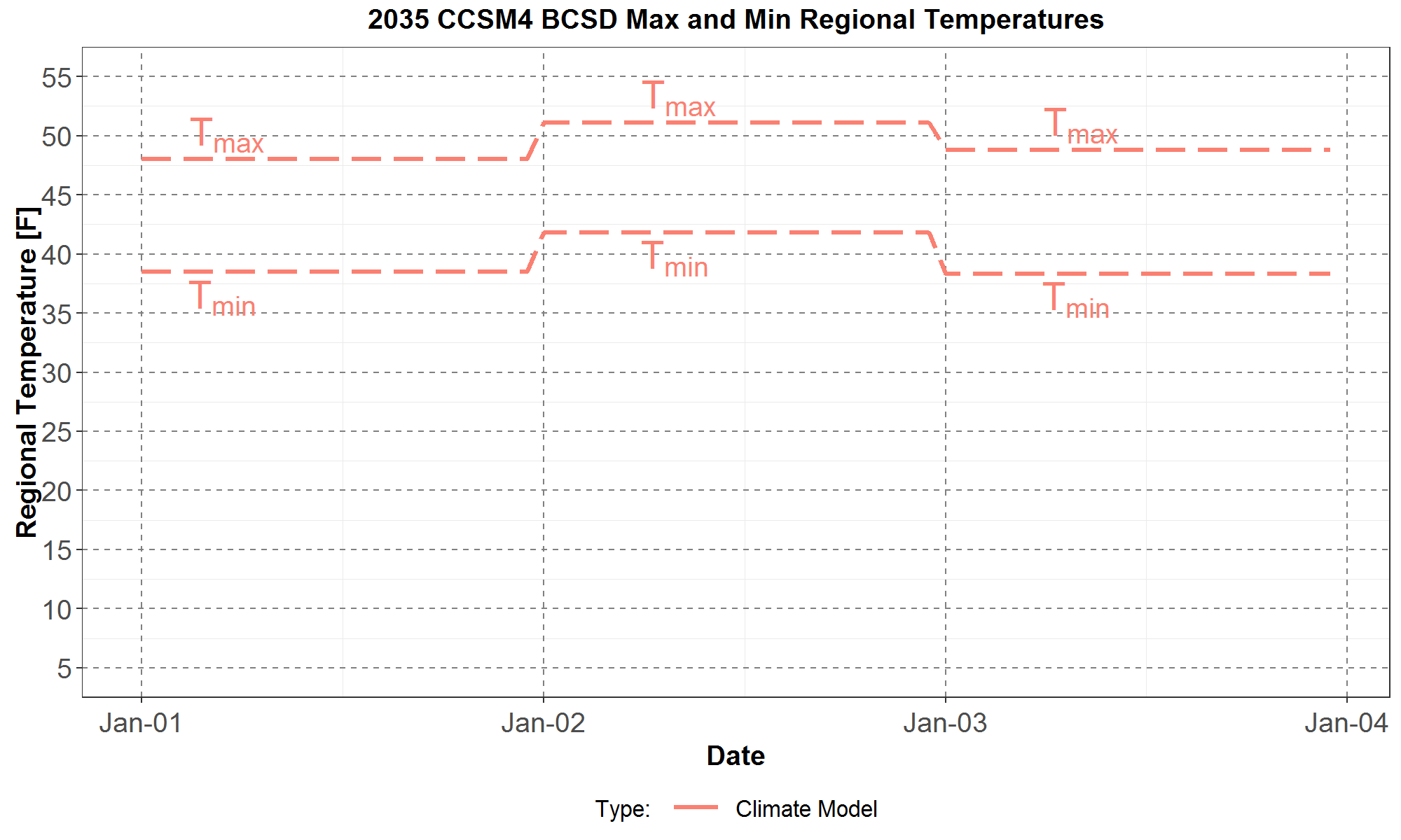
Figure 1: The daily minimum (Tmin) and maximum (Tmax) temperatures for the climate model CCSM4 with RCP 8.5 and BCSD downscaling method for January 1 to January 3 for the year 2035.
Figure 1 shows that for January 1, 2035, the minimum and maximum regional CCSM4 temperatures are 38.5 F and 48.0 F respectively, while for January 2, they are 41.8 F and 51.1 F respectively, and for January 3, they are 38.3 F and 48.8 F, respectively.
Next, historical regional hourly temperatures are used to transform the climate data forecasted regional daily minimum and maximum temperatures into hourly temperatures. As an example, the transformation method is demonstrated for the CCSM4 daily temperatures in Figure 1 by using the hourly shapes for each day from the historical year 1950. Thus, the example begins with the 1950 regional hourly temperatures for January 1 to January 3 plotted in Figure 2.
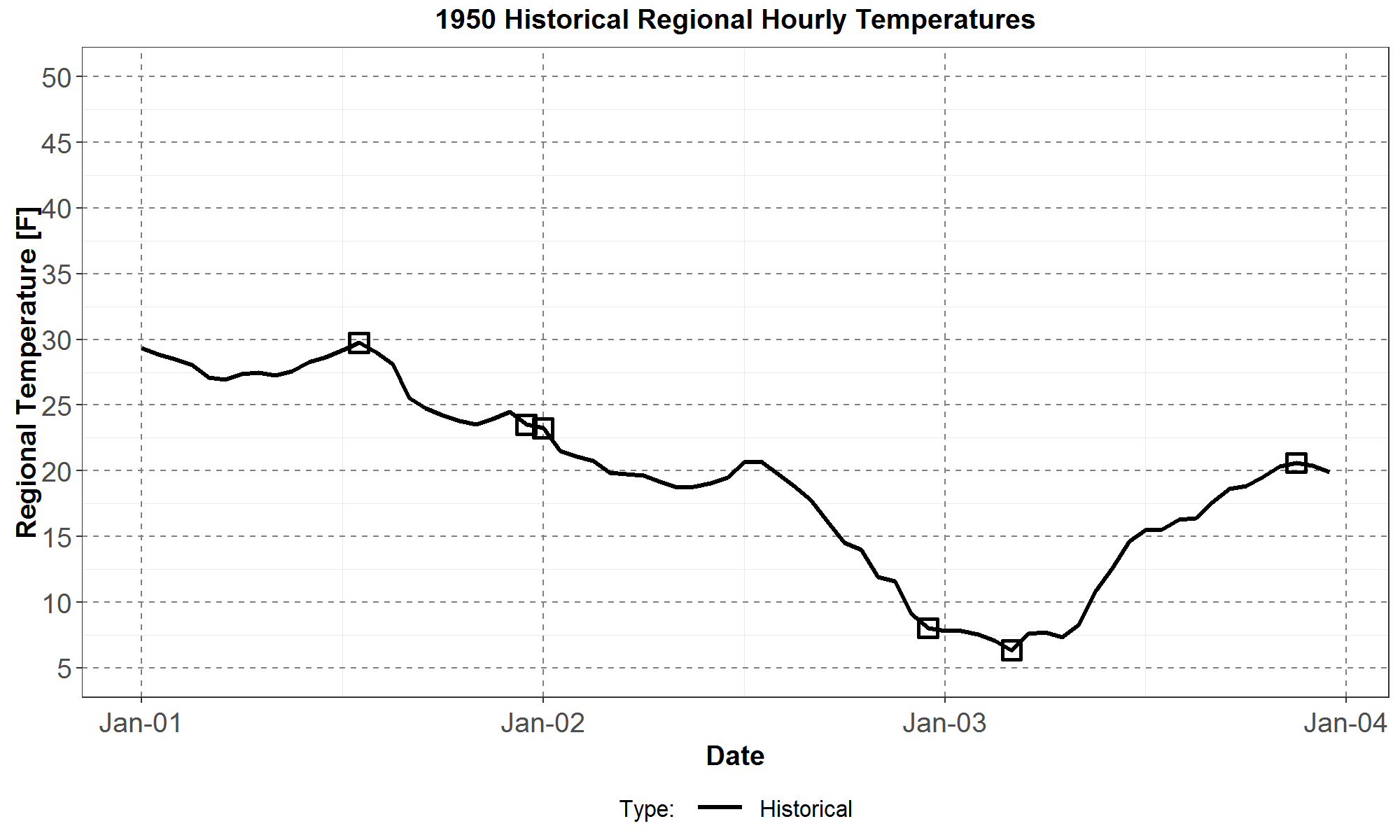
Figure 2: The historical regional hourly temperatures for January 1 to January 3 for the year 1950 in the black curve. The black open squares are the daily minimum and maximum temperatures.
On Figure 2, for January 1, the maximum temperature is 29.7 F and occurs at hour (starting) 13 while the minimum temperature is 23.5 F and occurs at hour 23. Similarly, for January 2, the maximum and minimum temperatures are 23.3 F and 8.0 F and take place at hours 0 and 23, respectively. And finally, for January 3, the maximum and minimum temperatures are 20.6 F and 6.3 F and occur respectively at hours 21 and 4.
As illustrated in Figure 3 below, our method assumes a transformation that maps the historical minimum and maximum temperatures (black squares) to the corresponding climate model minimum and maximum temperatures (orange squares) at the same respective hours for each day.
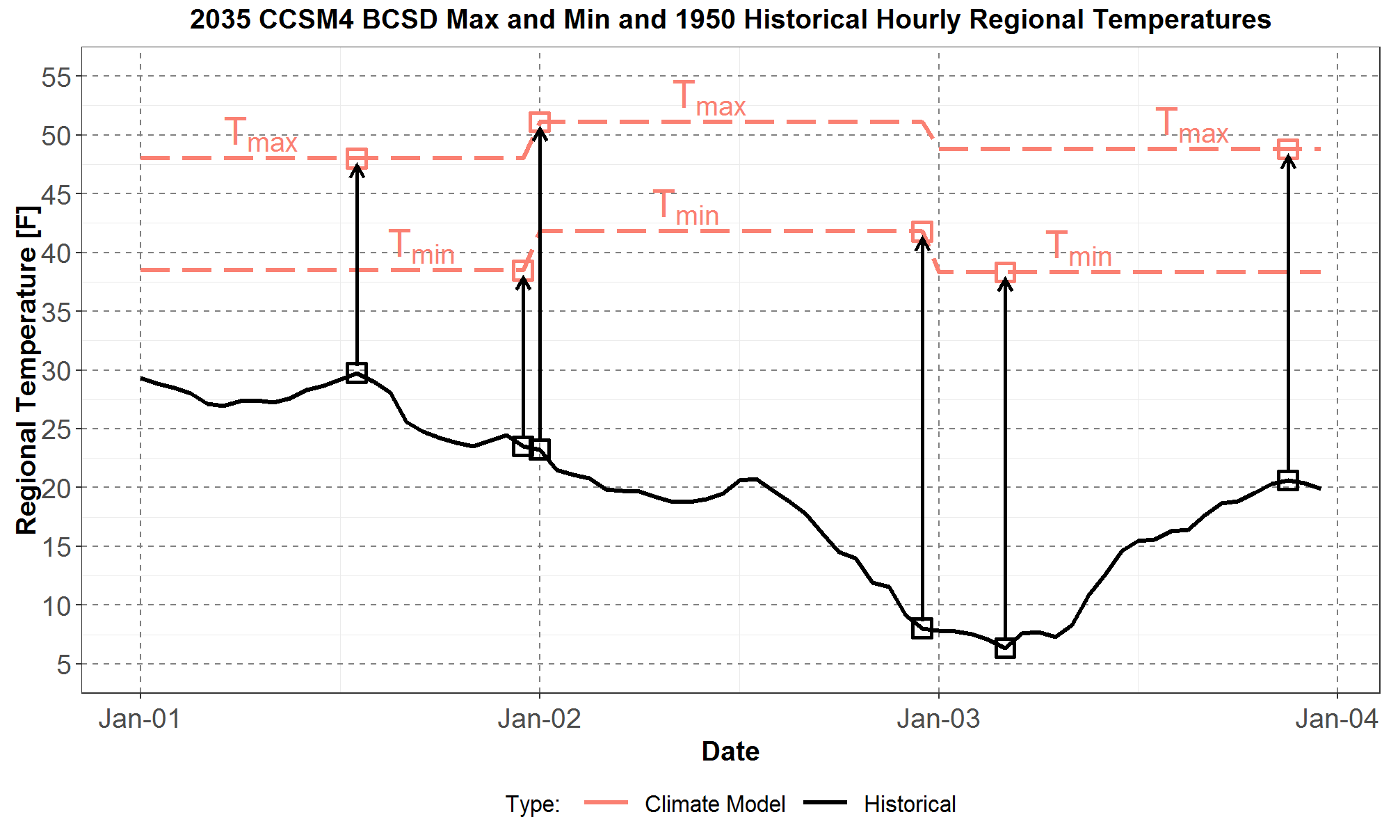
Figure 3: For January 1, the maximum historical temperature 29.7 (black square) is transformed to the maximum CCSM4 temperature 37.6 (orange square) now specified to occur at hour 13, while the minimum historical temperature 23.5 (black square) is transformed to the minimum CCSM4 temperature 31.5 (orange square) to occur at hour 23. For January 2, the historical 23.3 (black square) is transformed to the CCSM4 39.2 (orange square) at hour 0, and the historical 8.0 (black square) is transformed to the CCSM4 30.3 (orange square) at hour 23. Finally, for January 3, the historical temperature set (20.6, 6.3) in black squares is transformed to the CCSM4 set (45.5, 35.5) in orange squares at hours 21 and 4, respectively.
More explicitly, a linear transformation is used to map the historical minimum and maximum to the corresponding CCSM4 minimum and maximum. For example, for January 1, the linear transformation is
| αJan-1(29.7)+βJan-1=48.0 | (2) | |
| αJan-1(23.5)+βJan-1=38.5 | (3) |
with parameters αJan-1 and βJan-1 . The solution to Equations (2) and (3), to 3 significant figures, is αJan-1= 1.53 , and βJan-1 = 2.55.
Similarly, for January 2, the linear transformation is
| αJan-2(23.3)+βJan-2=51.1 | (4) | |
| αJan-2(8.0)+βJan-2 =41.8 | (5) |
with parameters αJan-2 and βJan-2 . The solution to Equations (4) and (5), is αJan-2= 0.612 , and βJan-2 = 36.9.
Finally, for January 3, the linear transformation from historical minimum and maximum temperatures to the respective CCSM4 minimum and maximum temperatures is
| αJan-3(20.6)+βJan-3=48.8 | (6) | |
| αJan-3(6.3)+βJan-3 =38.3 | (7) |
which leads to αJan-3= 0.734 , and βJan-3 = 33.7.
Therefore, for January 1 to 3, the three sets of parameters, (αJan-1 , βJan-1), (αJan-2 , βJan-2) and (αJan-3 , βJan-3) are used to transform the historical minimum and maximum temperatures to the corresponding CCSM4 minimum and maximum temperatures, for the same hours as the historical data. The equations above can then also be used to transform the remaining 22 hours of historical hourly temperatures into CCSM4 hourly temperatures for each day, as illustrated in Figure 4 below.
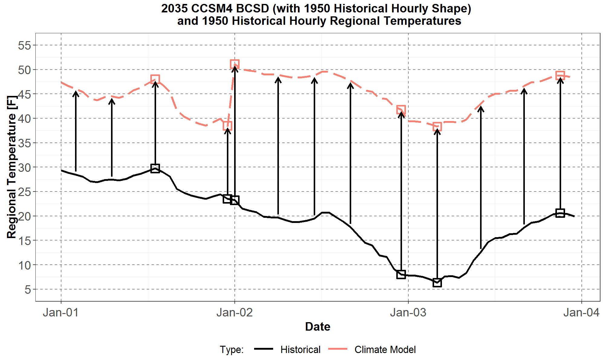
Figure 4: For January 1 to January 3, the 1950 historical hourly temperatures for January 1 to January 3 in the solid black curve are transformed to the 2035 CCSM4 hourly temperatures in the dashed orange curve using parameters (αJan-1 , βJan-1), (αJan-2 , βJan-2) and (αJan-3 , βJan-3) respectively.
In this example, the orange dashed curve in Figure 4 represents what the 2035 CCSM4 hourly temperatures would be given the CCSM4 daily minimum and maximum temperatures (orange squares) and the 1950 historical hourly shapes for January 1 to 3. However, this transformation sometimes introduces a significant step-change in temperature (or equivalently a discontinuity in the slope) between the last hour of a day and the first hour of the next day as observed between Jan 1 and Jan 2 in Figure 4. Nevertheless, for each of remaining 362 days of the year, the same type of linear transformation, as expressed in Equations (2) and (3), could also be used to calculate the 2035 CCSM4 hourly temperatures with the 1950 historical hourly temperature shape for the same day. It should be noted that the linear transformation in Equations (2) and (3) becomes singular and thus has no solution for parameters α and β if the historical minimum and maximum temperatures are the same, in other words, if the historical temperatures are constant for the day of interest. Fortunately, for all 71 years (from 1948 to 2018) of historical hourly temperatures, there is no day for which the temperatures are constant.
The next step then is applying the transformation to the CCSM4 minimum and maximum daily temperatures for January 1 to 3 using all 71 years of historical hourly temperature shapes, as shown in the 71 orange traces in Figure 5.
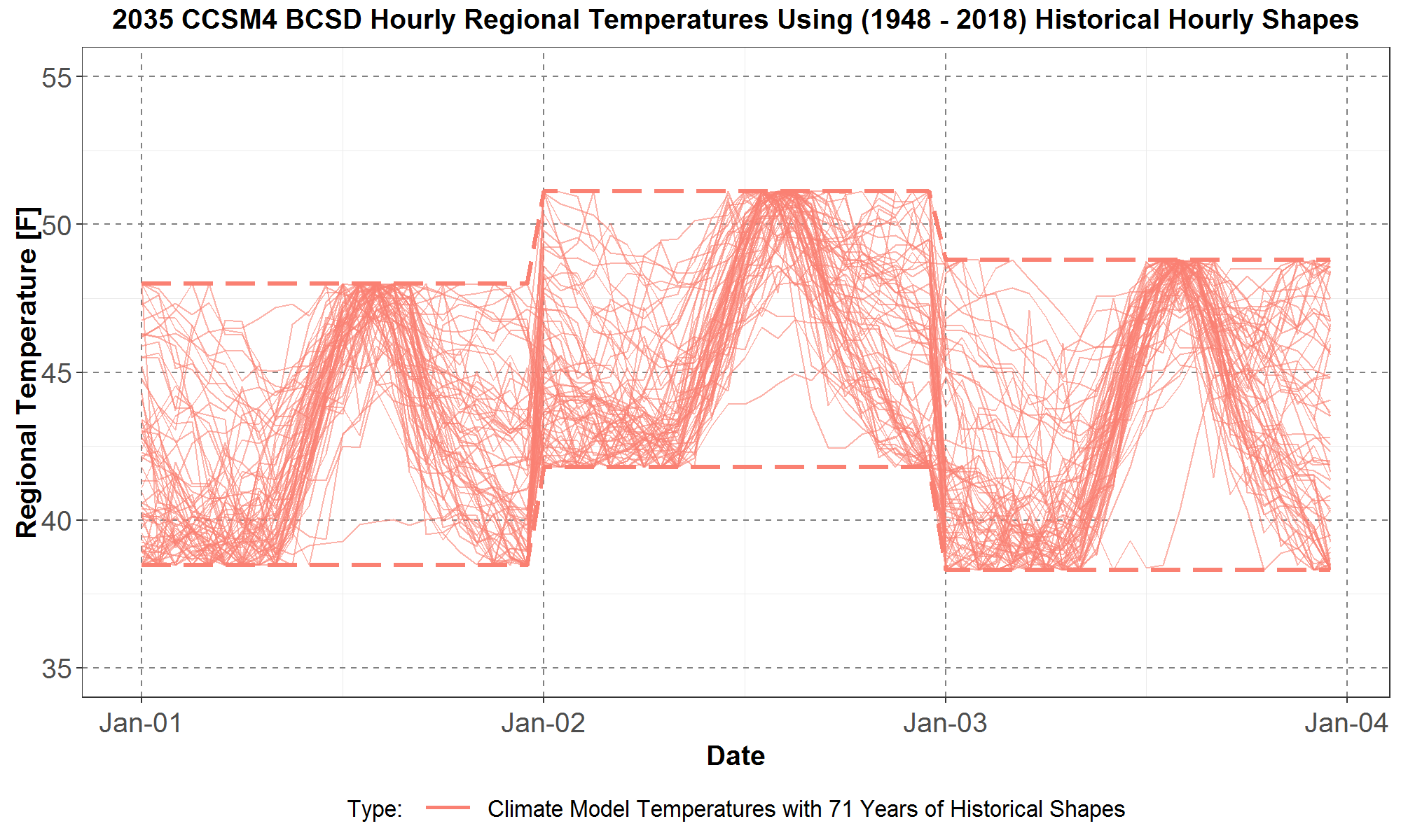
Figure 5: For January 1 to January 3, the 2035 CCSM4 hourly temperatures with the 1948 to 2018 (71 years) historical hourly temperature shapes are plotted in the 71 orange traces. All 71 traces are obtained using similar linear transformations as those in Equations (2) to (7), and all have the same 2035 CCSM4 daily minimum and maximum temperatures, as plotted in the orange dashed curves.
Figure 5 shows that for January 1 to January 3, all 71 traces have the same 2035 CCSM4 daily minimum and maximum temperatures as plotted in the orange dashed curves. And because the 71 years of historical hourly shapes are different, the minimum and maximum temperatures occur at many different hours of the day, as seen in Figure 5.
Unfortunately, it is impractical to use all 71 historical hourly temperature shapes for every future climate year from 2020 to 2049 for all 19 RMJOC climate scenarios (see RMJOC report I), even though for the 2021 Power Plan, only a small subset of the climate scenarios will be used. Therefore, one representative historical year is chosen from which to calculate hourly shapes for the daily climate temperatures for those scenarios selected for the plan.
An initial idea was to use the average hourly temperatures from the 71-year historical record. The resulting average hourly temperatures for CCSM4 are plotted in Figure 6, as represented by the blue dashed curve.
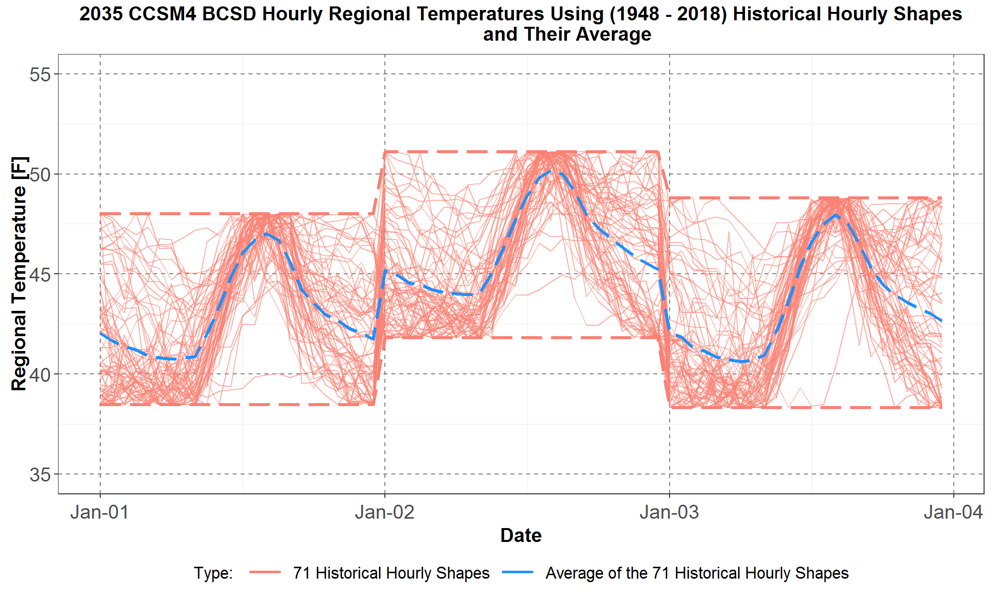
Figure 6: For January 1 to January 3, the 2035 CCSM4 hourly temperatures having the 1948 to 2018 (71 years) historical hourly temperature shapes are plotted in the orange traces. The blue dashed curve is the average of the 71 orange traces.
However, as seen in Figure 6, the average hourly temperatures do not have the same 2035 CCSM4 daily minimum and maximum temperatures (the orange dashed curves) and thus are not an appropriate representation of the 2035 CCSM4 temperatures. But even though these calculated hourly temperatures do not have the correct daily minimum and maximum temperatures, the resultant hourly shape looks reasonable, and thus it could perhaps be used to find a representative shape for the 2035 CCSM4 hourly temperatures.
The method then is to find a representative hourly shape, among the set of 71 orange traces, that is closest to the blue dashed curve. The procedure is as follows: for each orange trace, calculate the absolute value of the difference between its hourly temperature and the average hourly temperature (blue dashed curve) for all 8760 hours of the year, and then take the sum of all the absolute values. The trace with the minimum sum will be defined as being closest to the blue dashed curve. From the 71 traces for the 2035 CCSM4 hourly temperatures in Figure 6, the trace for year-1987 is the closest to the average. The results are plotted in Figure 7.
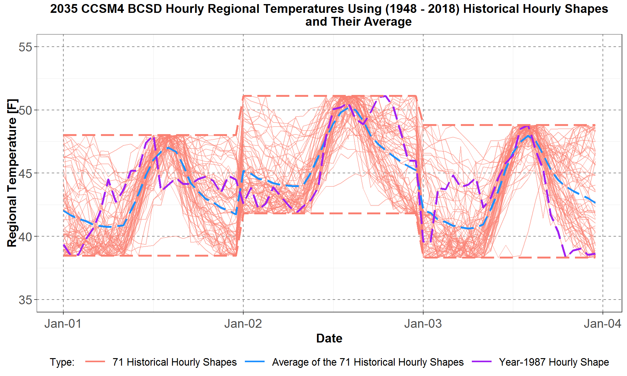
Figure 7: For January 1 to January 3, the 2035 CCSM4 hourly temperatures having the 1948 to 2018 (71 years) historical hourly temperature shapes are plotted in the orange traces. The blue dashed curve is the average of the 71 orange traces. The year-1987 orange trace is plotted as the purple dashed curve, and it has the minimum sum over 8760 hours of the absolute values of the difference between its temperature and the average temperature (in the blue dashed curve).
Therefore, in Figure 7, the CCSM4 hourly temperatures having year-1987 historical hourly shapes, plotted in the purple dashed curve, will serve as the best representative, from the 71 orange traces, for the CCSM4 hourly temperatures.
The method described above to calculate representative hourly shapes for the downscaled CCSM4_BCSD daily temperatures for year-2035 was also applied to all other future years from 2020 to 2049. In addition, the method was also used for the rest of the twenty downscaled GCMs listed in Table 2. Results show that the historical year-1987 hourly temperature shape is also the closest trace to the 71-year averaged curve for every future year from 2020 to 2049 in all twenty downscaled GCMs. Thus, the year-1987 historical hourly temperature shape will be used to transform the daily temperatures to hourly temperatures for all downscaled GCMs (or climate scenarios) used in the power plan.
The climate hourly temperatures, transformed from daily temperatures using year-1987 historical hourly shape, are used to select a subset of the RMJOC climate scenarios for study in the 2021 Power Plan. Furthermore, these hourly temperatures are also used as input in the short-term load forecasting model.